这个系列目的是揭开嵌入的神秘面纱,并展示如何在你的项目中使用它们。第一篇博客 介绍了如何使用和扩展开源嵌入模型,选择现有的模型,当前的评价方法,以及生态系统的发展状态。第二篇博客将会更一步深入嵌入并解释双向编码和交叉编码的区别。进一步我们将了解 检索和重排序 的理论。我们会构建一个工具,它可以来回答大约 400 篇 AI 的论文的问题。我们会在末尾大致讨论一下两个不同的论文。
你可以在这里阅读,或者通过点击左上角的图标在 Google Colab 中运行。现在我们正式开始学习!
简短概述
Sentence Transformers 支持两种类型的模型: Bi-encoders 和 Cross-encoders。Bi-encoders 更快更可扩展,但 Cross-encoders 更准确。虽然两者都处理类似的高水平任务,但何时使用一个而不是另一个是相当不同的。Bi-encoders 更适合搜索,而 Cross-encoders 更适合分类和高精度排序。下面讲下细节
介绍
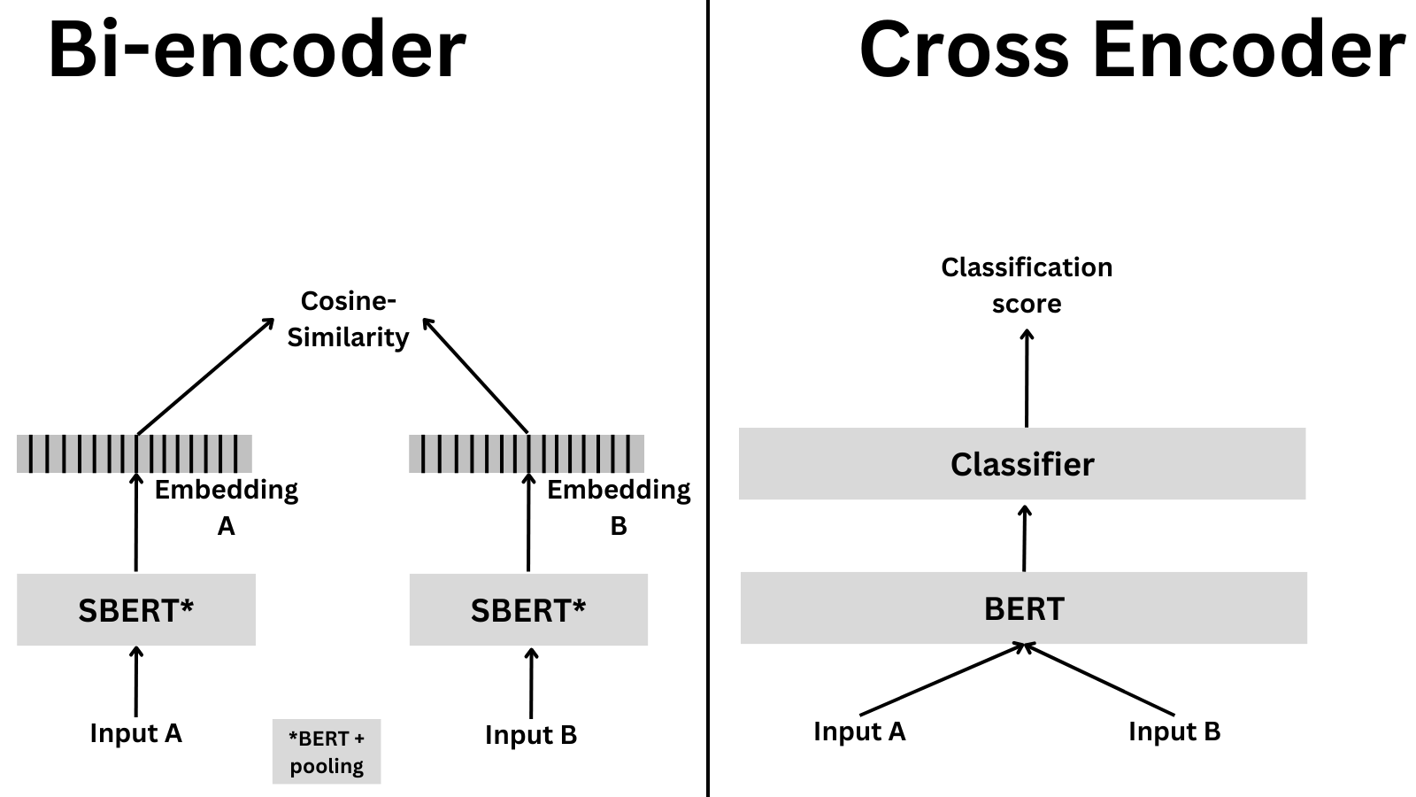
我们之前见过的模型都是双向编码器。双向编码器将输入文本编码成固定长度的向量。当我们计算两个句子的相似性时,我们通常将两个句子编码成两个向量,然后计算它们之间的相似性 (比如,使用余弦相似度)。我们训练双向编码器去优化,使得在问题和相关句子之间的相似度增加,而在其他句子之间的相似度减少。这也解释了为啥双向编码器更适合搜索。正如之前博客所说,双向编码器非常快,并且易于扩展。如果提供多个句子,双向编码器会独立编码每个句子。这意味着每个句子嵌入是互相独立的。这对于搜索来书是好的,因为我们可以并行编码数百万的句子。然而,这同样意味着双向编码器不知道任何关于句子之间的关系的知识。
当我们使用交叉编码,就会有所不同。交叉编码同时编码两个句子,并且输出一个分类分数。图示展示了它们之间的区别。
为啥使用这个而不用其他的?交叉编码更慢并且需要更多的内存,但同样更精确。一个交叉编码器对于比较几十个句子是一个很好的选择。如果我们要比较成千上万个句子,一个双向编码器是更好的选择,因为否则的话,它将会非常慢。如果你更在乎精度并且想高效的比较成千上万个句子呢?这有个当你想要检索信息的经典示例,在那个示例中,一个选择是首先使用双向编码器去减少候选数量 (比如,获取最相关的 20 个例子),然后使用交叉编码器获得最终结果。这个也叫做重排序,在信息检索中是一个常用的技术。我们将在后面学习更多关于这个的内容。
由于交叉编码更精确,它同样适用于一些微小差异很重要的任务,比如医疗或者法律文档,其中一点微小的差异可以改变句子的整个意思。
交叉编码器
正如之前所说,交叉编码器同时编码两个句子,并输出一个分类标签。交叉编码器第一次生成一个单独的嵌入,它捕获了句子的表征和相关关系。与双向编码器生成的嵌入 (它们是独立的) 不同,交叉编码器是互相依赖的。这也是为什么交叉编码器更适合分类,并且其质量更高,他们可以捕获两个句子之间的关系!反过来说,如果你需要比较上千个句子的话,交叉编码器会很慢,因为他们要编码所有的句子对。
假如你有四个句子,并且你需要比较所有的可能对:
- 一个双向编码器需要独立编码每个句子,所以它需要编码四个句子。
- 一个交叉编码器需要同时编码所的句子对,所以它需要编码六个句子对 (AB, AC, AD, BC, BD, CD)。
让我们再扩展一下,如果你要 100,000 个句子,并且你需要比较所有的可能对:
- 一个双向编码器需要编码 100,000 个句子。
- 一个交叉编码器需要编码 4,999,950,000 个句子对。(用 组合数公式:
n! / (r!(n-r)!), 这里面 n = 100,000, r = 2) 所以扩展并不好
也难怪他们会更慢!
尽管交叉编码器再分类层前有一个适度的嵌入,但这并没有用于相似性搜索。这是因为交叉编码器被训练来优化分类损失,而不是相似性损失。因此,嵌入是针对分类任务而设计的,并且不用于相似性任务。
他们可以被用于不同的任务。例如,对于段落检索 (给定一个问题和一个段落,段落是否与问题相关)。让我们看一个快速代码片段,使用一个小的交叉编码模型训练这个:
!pip install sentence_transformers datasets
from sentence_transformers import CrossEncoder

model = CrossEncoder('cross-encoder/ms-marco-TinyBERT-L-2-v2', max_length=512)
scores = model.predict([('How many people live in Berlin?', 'Berlin had a population of 3,520,031 registered inhabitants in an area of 891.82 square kilometers.'),
                        ('How many people live in Berlin?', 'Berlin is well known for its museums.')])
scores
array([ 7.152365 , -6.2870445], dtype=float32)
另一个用例,用交叉编码做语义相似度,跟我们用双向编码器的结果很相似。比如,给定两个句子,他们语义上相似吗?尽管这个任务跟我们用双向编码器解决的任务是一样的,但是交叉编码器更准确,更慢。
model = CrossEncoder('cross-encoder/stsb-TinyBERT-L-4')
scores = model.predict([("The weather today is beautiful", "It's raining!"),
                        ("The weather today is beautiful", "Today is a sunny day")])
scores
array([0.46552283, 0.6350213 ], dtype=float32)
检索和重排序
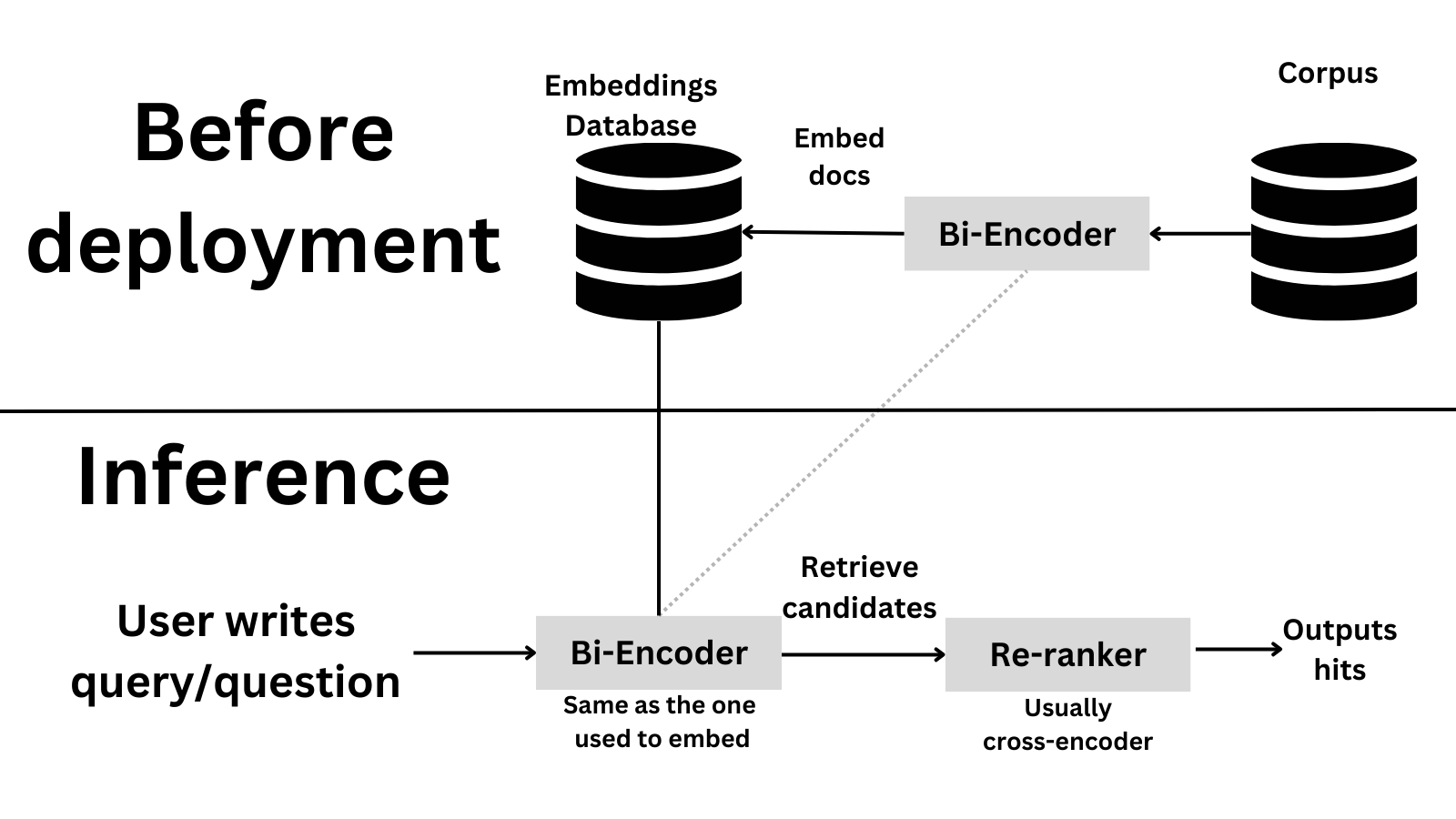
现在我们已经了解了交叉编码器和双向编码器的不同,让我们看看如何使在实践中用它们来构建一个检索和重排序系统。这是一个常见的信息检索技巧,首先检索最相关的文档然后用一个更精确的模型进行重排序。这对于高效比较成千个句子的查询是个不错的选择并且更加注重精度。
假设你有一个有 100,000 个句子的语料库并且想要对给定查询找到最相关的句子。第一步就是使用双向编码器去检索很多候选 (为了确保召回)。然后,使用交叉编码器去重新排序候选并且得到最终的带有高精度的结果。这是高层次上看这个系统的样子
让我们试一试执行一个论文搜索系统!我们将使用一个 AI Arxiv 数据集,这个是在 Pinecone 上关于重排序极好的教程 。其目的是问 AI 一个 问题,我们获得最相关的论文部分并且回答问题。
from datasets import load_dataset

dataset = load_dataset("jamescalam/ai-arxiv-chunked")
dataset["train"]
Found cached dataset json (/home/osanseviero/.cache/huggingface/datasets/jamescalam___json/jamescalam--ai-arxiv-chunked-0d76bdc6812ffd50/0.0.0/8bb11242116d547c741b2e8a1f18598ffdd40a1d4f2a2872c7a28b697434bc96)
 0%|          | 0/1 [00:00<?, ?it/s]
Dataset({
    features: ['doi', 'chunk-id', 'chunk', 'id', 'title', 'summary', 'source', 'authors', 'categories', 'comment', 'journal_ref', 'primary_category', 'published', 'updated', 'references'],
    num_rows: 41584
})
如果你检查了数据集,它是一个划分切块好的 400 篇 Arxiv 论文,切块意味着每个部分被分成更小的部分,以使模型更容易处理。这里是一个样本:
dataset["train"][0]
{'doi': '1910.01108',
 'chunk-id': '0',
 'chunk': 'DistilBERT, a distilled version of BERT: smaller,\nfaster, cheaper and lighter\nVictor SANH, Lysandre DEBUT, Julien CHAUMOND, Thomas WOLF\nHugging Face\n{victor,lysandre,julien,thomas}@huggingface.co\nAbstract\nAs Transfer Learning from large-scale pre-trained models becomes more prevalent\nin Natural Language Processing (NLP), operating these large models in on-theedge and/or under constrained computational training or inference budgets remains\nchallenging. In this work, we propose a method to pre-train a smaller generalpurpose language representation model, called DistilBERT, which can then be finetuned with good performances on a wide range of tasks like its larger counterparts.\nWhile most prior work investigated the use of distillation for building task-specific\nmodels, we leverage knowledge distillation during the pre-training phase and show\nthat it is possible to reduce the size of a BERT model by 40%, while retaining 97%\nof its language understanding capabilities and being 60% faster. To leverage the\ninductive biases learned by larger models during pre-training, we introduce a triple\nloss combining language modeling, distillation and cosine-distance losses. Our\nsmaller, faster and lighter model is cheaper to pre-train and we demonstrate its',
 'id': '1910.01108',
 'title': 'DistilBERT, a distilled version of BERT: smaller, faster, cheaper and lighter',
 'summary': 'As Transfer Learning from large-scale pre-trained models becomes more\nprevalent in Natural Language Processing (NLP), operating these large models in\non-the-edge and/or under constrained computational training or inference\nbudgets remains challenging. In this work, we propose a method to pre-train a\nsmaller general-purpose language representation model, called DistilBERT, which\ncan then be fine-tuned with good performances on a wide range of tasks like its\nlarger counterparts. While most prior work investigated the use of distillation\nfor building task-specific models, we leverage knowledge distillation during\nthe pre-training phase and show that it is possible to reduce the size of a\nBERT model by 40%, while retaining 97% of its language understanding\ncapabilities and being 60% faster. To leverage the inductive biases learned by\nlarger models during pre-training, we introduce a triple loss combining\nlanguage modeling, distillation and cosine-distance losses. Our smaller, faster\nand lighter model is cheaper to pre-train and we demonstrate its capabilities\nfor on-device computations in a proof-of-concept experiment and a comparative\non-device study.',
 'source': 'http://arxiv.org/pdf/1910.01108',
 'authors': ['Victor Sanh',
  'Lysandre Debut',
  'Julien Chaumond',
  'Thomas Wolf'],
 'categories': ['cs.CL'],
 'comment': 'February 2020 - Revision: fix bug in evaluation metrics, updated\n  metrics, argumentation unchanged. 5 pages, 1 figure, 4 tables. Accepted at\n  the 5th Workshop on Energy Efficient Machine Learning and Cognitive Computing\n  - NeurIPS 2019',
 'journal_ref': None,
 'primary_category': 'cs.CL',
 'published': '20191002',
 'updated': '20200301',
 'references': [{'id': '1910.01108'}]}
让我们获得所有的切块,然后编码:
chunks = dataset["train"]["chunk"]
len(chunks)
41584
现在,我们将使用一个双向编码器来编码所有的切块到嵌入。我们将会截断过长的段落,最大不超过 512 token。注意,短文本是许多嵌入模型的缺点之一!我们将会特别使用 multi-qa-MiniLM-L6-cos-v1 模型。这是一个小模型,用来训练把问题和段落编码成小的嵌入空间。因为这是一个双向编码器模型,所以很快和易扩展。
在我这个普通的电脑上嵌入所有的 40,000+ 文章大概需要 30 秒。注意,我们只要嵌入一次,然后可以保存到磁盘并且之后加载。在生产环境中,你可以把嵌入保存到数据库中并从中加载嵌入。
from sentence_transformers import SentenceTransformer

bi_encoder = SentenceTransformer('multi-qa-MiniLM-L6-cos-v1')
bi_encoder.max_seq_length = 256

corpus_embeddings = bi_encoder.encode(chunks, convert_to_tensor=True, show_progress_bar=True)
Batches: 0%| | 0/1300 [00:00<?, ?it/s]
真棒!现在,让我们试一个问题,搜索其相关文章。为了做到这一点,我们需要编码问题,然后计算问题和所有段落之间的相似度。开干,看看前几个结果!
from sentence_transformers import util

query = "what is rlhf?"
top_k = 25 # how many chunks to retrieve
query_embedding = bi_encoder.encode(query, convert_to_tensor=True).cuda()

hits = util.semantic_search(query_embedding, corpus_embeddings, top_k=top_k)[0]
hits
[{'corpus_id': 14679, 'score': 0.6097552180290222},
 {'corpus_id': 17387, 'score': 0.5659530162811279},
 {'corpus_id': 39564, 'score': 0.5590510368347168},
 {'corpus_id': 14725, 'score': 0.5585878491401672},
 {'corpus_id': 5628, 'score': 0.5296251773834229},
 {'corpus_id': 14802, 'score': 0.5075011253356934},
 {'corpus_id': 9761, 'score': 0.49943411350250244},
 {'corpus_id': 14716, 'score': 0.4931946098804474},
 {'corpus_id': 9763, 'score': 0.49280521273612976},
 {'corpus_id': 20638, 'score': 0.4884325861930847},
 {'corpus_id': 20653, 'score': 0.4873950183391571},
 {'corpus_id': 9755, 'score': 0.48562008142471313},
 {'corpus_id': 14806, 'score': 0.4792214035987854},
 {'corpus_id': 14805, 'score': 0.475425660610199},
 {'corpus_id': 20652, 'score': 0.4740477204322815},
 {'corpus_id': 20711, 'score': 0.4703512489795685},
 {'corpus_id': 20632, 'score': 0.4695567488670349},
 {'corpus_id': 14750, 'score': 0.46810320019721985},
 {'corpus_id': 14749, 'score': 0.46809980273246765},
 {'corpus_id': 35209, 'score': 0.46695172786712646},
 {'corpus_id': 14671, 'score': 0.46657535433769226},
 {'corpus_id': 14821, 'score': 0.4637290835380554},
 {'corpus_id': 14751, 'score': 0.4585301876068115},
 {'corpus_id': 14815, 'score': 0.45775431394577026},
 {'corpus_id': 35250, 'score': 0.4569615125656128}]
#Let's store the IDs for later
retrieval_corpus_ids = [hit['corpus_id'] for hit in hits]

# Now let's print the top 3 results
for i, hit in enumerate(hits[:3]):
    sample = dataset["train"][hit["corpus_id"]]
    print(f"Top {i+1} passage with score {hit['score']} from {sample['source']}:")
    print(sample["chunk"])
    print("\n")
Top 1 passage with score 0.6097552180290222 from http://arxiv.org/pdf/2204.05862:
learning from human feedback, which we improve on a roughly weekly cadence. See Section 2.3.
4This means that our helpfulness dataset goes ‘up’ in desirability during the conversation, while our harmlessness
dataset goes ‘down’ in desirability. We chose the latter to thoroughly explore bad behavior, but it is likely not ideal
for teaching good behavior. We believe this difference in our data distributions creates subtle problems for RLHF, and
suggest that others who want to use RLHF to train safer models consider the analysis in Section 4.4.
5
1071081091010
Number of Parameters0.20.30.40.50.6Mean Eval Acc
Mean Zero-Shot Accuracy
Plain Language Model
RLHF
1071081091010
Number of Parameters0.20.30.40.50.60.7Mean Eval Acc
Mean Few-Shot Accuracy
Plain Language Model
RLHFFigure 3 RLHF model performance on zero-shot and few-shot NLP tasks. For each model size, we plot
the mean accuracy on MMMLU, Lambada, HellaSwag, OpenBookQA, ARC-Easy, ARC-Challenge, and
TriviaQA. On zero-shot tasks, RLHF training for helpfulness and harmlessness hurts performance for small


Top 2 passage with score 0.5659530162811279 from http://arxiv.org/pdf/2302.07842:
preferences and values which are difficult to capture by hard- coded reward functions.
RLHF works by using a pre-trained LM to generate text, which i s then evaluated by humans by, for example,
ranking two model generations for the same prompt. This data is then collected to learn a reward model
that predicts a scalar reward given any generated text. The r eward captures human preferences when
judging model output. Finally, the LM is optimized against s uch reward model using RL policy gradient
algorithms like PPO ( Schulman et al. ,2017). RLHF can be applied directly on top of a general-purpose LM
pre-trained via self-supervised learning. However, for mo re complex tasks, the model’s generations may not
be good enough. In such cases, RLHF is typically applied afte r an initial supervised fine-tuning phase using
a small number of expert demonstrations for the correspondi ng downstream task ( Ramamurthy et al. ,2022;
Ouyang et al. ,2022;Stiennon et al. ,2020).
A successful example of RLHF used to teach a LM to use an extern al tool stems from WebGPT Nakano et al.
(2021) (discussed in 3.2.3), a model capable of answering questions using a search engine and providing


Top 3 passage with score 0.5590510368347168 from http://arxiv.org/pdf/2307.09288:
31
5 Discussion
Here, we discuss the interesting properties we have observed with RLHF (Section 5.1). We then discuss the
limitations of L/l.sc/a.sc/m.sc/a.sc /two.taboldstyle-C/h.sc/a.sc/t.sc (Section 5.2). Lastly, we present our strategy for responsibly releasing these
models (Section 5.3).
5.1 Learnings and Observations
Our tuning process revealed several interesting results, such as L/l.sc/a.sc/m.sc/a.sc /two.taboldstyle-C/h.sc/a.sc/t.sc ’s abilities to temporally
organize its knowledge, or to call APIs for external tools.
SFT (Mix)
SFT (Annotation)
RLHF (V1)
0.0 0.2 0.4 0.6 0.8 1.0
Reward Model ScoreRLHF (V2)
Figure 20: Distribution shift for progressive versions of L/l.sc/a.sc/m.sc/a.sc /two.taboldstyle-C/h.sc/a.sc/t.sc , from SFT models towards RLHF.
Beyond Human Supervision. At the outset of the project, many among us expressed a preference for
好极了!我们根据最高召回但低精度的双向编码器得到了最相似的切块。
现在,让我们通过高精度的交叉编码器模型重排序。我们将使用 cross-encoder/ms-marco-MiniLM-L-6-v2 模型。这个模型是在 MS MARCO 数据集上微调的,它是一个大型真实问答信息检索数据集。这使得这个模型在进行问答时非常适合决策。
我们将使用同样的问题和我们从双向编码器获得的前 10 个块。让我们看看结果!回想一下,交叉编码器需要成对的,所以我们将创建问题和每个块的对。
from sentence_transformers import  CrossEncoder
cross_encoder = CrossEncoder('cross-encoder/ms-marco-MiniLM-L-6-v2')

cross_inp = [[query, chunks[hit['corpus_id']]] for hit in hits]
cross_scores = cross_encoder.predict(cross_inp)
cross_scores
array([ 1.2227577 ,  5.048051  ,  1.2897239 ,  2.205767  ,  4.4136825 ,
        1.2272772 ,  2.5638275 ,  0.81847703,  2.35553   ,  5.590804  ,
        1.3877895 ,  2.9497519 ,  1.6762824 ,  0.7211323 ,  0.16303705,
        1.3640019 ,  2.3106787 ,  1.5849439 ,  2.9696884 , -1.1079378 ,
        0.7681126 ,  1.5945492 ,  2.2869687 ,  3.5448399 ,  2.056368  ],
      dtype=float32)
让我们增加一个新的属性 cross-score ,并将其排序!
for idx in range(len(cross_scores)):
    hits[idx]['cross-score'] = cross_scores[idx]
hits = sorted(hits, key=lambda x: x['cross-score'], reverse=True)
msmarco_l6_corpus_ids = [hit['corpus_id'] for hit in hits] # save for later

hits
[{'corpus_id': 20638, 'score': 0.4884325861930847, 'cross-score': 5.590804},
 {'corpus_id': 17387, 'score': 0.5659530162811279, 'cross-score': 5.048051},
 {'corpus_id': 5628, 'score': 0.5296251773834229, 'cross-score': 4.4136825},
 {'corpus_id': 14815, 'score': 0.45775431394577026, 'cross-score': 3.5448399},
 {'corpus_id': 14749, 'score': 0.46809980273246765, 'cross-score': 2.9696884},
 {'corpus_id': 9755, 'score': 0.48562008142471313, 'cross-score': 2.9497519},
 {'corpus_id': 9761, 'score': 0.49943411350250244, 'cross-score': 2.5638275},
 {'corpus_id': 9763, 'score': 0.49280521273612976, 'cross-score': 2.35553},
 {'corpus_id': 20632, 'score': 0.4695567488670349, 'cross-score': 2.3106787},
 {'corpus_id': 14751, 'score': 0.4585301876068115, 'cross-score': 2.2869687},
 {'corpus_id': 14725, 'score': 0.5585878491401672, 'cross-score': 2.205767},
 {'corpus_id': 35250, 'score': 0.4569615125656128, 'cross-score': 2.056368},
 {'corpus_id': 14806, 'score': 0.4792214035987854, 'cross-score': 1.6762824},
 {'corpus_id': 14821, 'score': 0.4637290835380554, 'cross-score': 1.5945492},
 {'corpus_id': 14750, 'score': 0.46810320019721985, 'cross-score': 1.5849439},
 {'corpus_id': 20653, 'score': 0.4873950183391571, 'cross-score': 1.3877895},
 {'corpus_id': 20711, 'score': 0.4703512489795685, 'cross-score': 1.3640019},
 {'corpus_id': 39564, 'score': 0.5590510368347168, 'cross-score': 1.2897239},
 {'corpus_id': 14802, 'score': 0.5075011253356934, 'cross-score': 1.2272772},
 {'corpus_id': 14679, 'score': 0.6097552180290222, 'cross-score': 1.2227577},
 {'corpus_id': 14716, 'score': 0.4931946098804474, 'cross-score': 0.81847703},
 {'corpus_id': 14671, 'score': 0.46657535433769226, 'cross-score': 0.7681126},
 {'corpus_id': 14805, 'score': 0.475425660610199, 'cross-score': 0.7211323},
 {'corpus_id': 20652, 'score': 0.4740477204322815, 'cross-score': 0.16303705},
 {'corpus_id': 35209, 'score': 0.46695172786712646, 'cross-score': -1.1079378}]
你可以从上面的数据看到,交叉编码器的结果和双向编码器的结果并不一致。神奇的是,一些最前面的交叉编码器结果 (14815 和 14749) 的结果其有着最低的双向编码器分数。这很合理,因为双向编码器比较的是问题和文档在嵌入空间的相似性,但交叉编码器考虑的是问题和文档在嵌入空间的相关性。
for i, hit in enumerate(hits[:3]):
    sample = dataset["train"][hit["corpus_id"]]
    print(f"Top {i+1} passage with score {hit['cross-score']} from {sample['source']}:")
    print(sample["chunk"])
    print("\n")
Top 1 passage with score 0.9668010473251343 from http://arxiv.org/pdf/2204.05862:
Stackoverflow Good Answer vs. Bad Answer Loss Difference
Python FT
Python FT + RLHF(b)Difference in mean log-prob between good and bad
answers to Stack Overflow questions.
Figure 37 Analysis of RLHF on language modeling for good and bad Stack Overflow answers, over many
model sizes, ranging from 13M to 52B parameters. Compared to the baseline model (a pre-trained LM
finetuned on Python code), the RLHF model is more capable of distinguishing quality (right) , but is worse
at language modeling (left) .
the RLHF models obtain worse loss. This is most likely due to optimizing a different objective rather than
pure language modeling.
B.8 Further Analysis of RLHF on Code-Model Snapshots
As discussed in Section 5.3, RLHF improves performance of base code models on code evals. In this appendix, we compare that with simply prompting the base code model with a sample of prompts designed to
elicit helpfulness, harmlessness, and honesty, which we refer to as ‘HHH’ prompts. In particular, they contain
a couple of coding examples. Below is a description of what this prompt looks like:
Below are a series of dialogues between various people and an AI assistant. The AI tries to be helpful,


Top 2 passage with score 0.9574587345123291 from http://arxiv.org/pdf/2302.07459:
We examine the influence of the amount of RLHF training for two reasons. First, RLHF [13, 57] is an
increasingly popular technique for reducing harmful behaviors in large language models [3, 21, 52]. Some of
these models are already deployed [52], so we believe the impact of RLHF deserves further scrutiny. Second,
previous work shows that the amount of RLHF training can significantly change metrics on a wide range of
personality, political preference, and harm evaluations for a given model size [41]. As a result, it is important
to control for the amount of RLHF training in the analysis of our experiments.
3.2 Experiments
3.2.1 Overview
We test the effect of natural language instructions on two related but distinct moral phenomena: stereotyping
and discrimination. Stereotyping involves the use of generalizations about groups in ways that are often
harmful or undesirable.4To measure stereotyping, we use two well-known stereotyping benchmarks, BBQ
[40] (§3.2.2) and Windogender [49] (§3.2.3). For discrimination, we focus on whether models make disparate
decisions about individuals based on protected characteristics that should have no relevance to the outcome.5
To measure discrimination, we construct a new benchmark to test for the impact of race in a law school course


Top 3 passage with score 0.9408788084983826 from http://arxiv.org/pdf/2302.07842:
preferences and values which are difficult to capture by hard- coded reward functions.
RLHF works by using a pre-trained LM to generate text, which i s then evaluated by humans by, for example,
ranking two model generations for the same prompt. This data is then collected to learn a reward model
that predicts a scalar reward given any generated text. The r eward captures human preferences when
judging model output. Finally, the LM is optimized against s uch reward model using RL policy gradient
algorithms like PPO ( Schulman et al. ,2017). RLHF can be applied directly on top of a general-purpose LM
pre-trained via self-supervised learning. However, for mo re complex tasks, the model’s generations may not
be good enough. In such cases, RLHF is typically applied afte r an initial supervised fine-tuning phase using
a small number of expert demonstrations for the correspondi ng downstream task ( Ramamurthy et al. ,2022;
Ouyang et al. ,2022;Stiennon et al. ,2020).
A successful example of RLHF used to teach a LM to use an extern al tool stems from WebGPT Nakano et al.
(2021) (discussed in 3.2.3), a model capable of answering questions using a search engine and providing
棒极了!这个结果似乎跟问题相关。我们还能做些什么来改进结果?
这里我们使用了 cross-encoder/ms-marco-MiniLM-L-6-v2, 这个模型已经有三年历史了,并且很小。它是 很多年前的最好的重新排序模型之一。
对于选择模型,我建议去 MTEB leaderboard,点击 reranking,选择一个适合你需求的模型。平均列可以很好地代表总体质量,但你可能对数据集特别感兴趣 (例如,检索选项卡中的 MSMarco)
注意,模型老模型,比如 MiniLM, 并不在那里。另外,并不是所有的模型都是交叉编码器,所以总是要实验,如果增加第二阶段,更慢的重新排序器是否值得。这里有一些有趣的发现:
- E5 Mistral 7B Instruct (2023 年 12 月): 这是一个基于解码器的嵌入 (不同于我们之前学的基于编码器的)。 这一点很有趣,因为使用解码器而不是编码器是一个新趋势,这样可以容纳更长的文本。这里是 相关论文
- BAAI Reranker (2023 年 9 月): 一个高质量重排序模型,其大小适中 (只有 278M 的参数)。让我们用这个模型获得结果并比较。
# Same code as before, just different model
cross_encoder = CrossEncoder('BAAI/bge-reranker-base')

cross_inp = [[query, chunks[hit['corpus_id']]] for hit in hits]
cross_scores = cross_encoder.predict(cross_inp)

for idx in range(len(cross_scores)):
    hits[idx]['cross-score'] = cross_scores[idx]

hits = sorted(hits, key=lambda x: x['cross-score'], reverse=True)
bge_corpus_ids = [hit['corpus_id'] for hit in hits]
for i, hit in enumerate(hits[:3]):
    sample = dataset["train"][hit["corpus_id"]]
    print(f"Top {i+1} passage with score {hit['cross-score']} from {sample['source']}:")
    print(sample["chunk"])
    print("\n")
Top 1 passage with score 0.9668010473251343 from http://arxiv.org/pdf/2204.05862:
Stackoverflow Good Answer vs. Bad Answer Loss Difference
Python FT
Python FT + RLHF(b)Difference in mean log-prob between good and bad
answers to Stack Overflow questions.
Figure 37 Analysis of RLHF on language modeling for good and bad Stack Overflow answers, over many
model sizes, ranging from 13M to 52B parameters. Compared to the baseline model (a pre-trained LM
finetuned on Python code), the RLHF model is more capable of distinguishing quality (right) , but is worse
at language modeling (left) .
the RLHF models obtain worse loss. This is most likely due to optimizing a different objective rather than
pure language modeling.
B.8 Further Analysis of RLHF on Code-Model Snapshots
As discussed in Section 5.3, RLHF improves performance of base code models on code evals. In this appendix, we compare that with simply prompting the base code model with a sample of prompts designed to
elicit helpfulness, harmlessness, and honesty, which we refer to as ‘HHH’ prompts. In particular, they contain
a couple of coding examples. Below is a description of what this prompt looks like:
Below are a series of dialogues between various people and an AI assistant. The AI tries to be helpful,


Top 2 passage with score 0.9574587345123291 from http://arxiv.org/pdf/2302.07459:
We examine the influence of the amount of RLHF training for two reasons. First, RLHF [13, 57] is an
increasingly popular technique for reducing harmful behaviors in large language models [3, 21, 52]. Some of
these models are already deployed [52], so we believe the impact of RLHF deserves further scrutiny. Second,
previous work shows that the amount of RLHF training can significantly change metrics on a wide range of
personality, political preference, and harm evaluations for a given model size [41]. As a result, it is important
to control for the amount of RLHF training in the analysis of our experiments.
3.2 Experiments
3.2.1 Overview
We test the effect of natural language instructions on two related but distinct moral phenomena: stereotyping
and discrimination. Stereotyping involves the use of generalizations about groups in ways that are often
harmful or undesirable.4To measure stereotyping, we use two well-known stereotyping benchmarks, BBQ
[40] (§3.2.2) and Windogender [49] (§3.2.3). For discrimination, we focus on whether models make disparate
decisions about individuals based on protected characteristics that should have no relevance to the outcome.5
To measure discrimination, we construct a new benchmark to test for the impact of race in a law school course


Top 3 passage with score 0.9408788084983826 from http://arxiv.org/pdf/2302.07842:
preferences and values which are difficult to capture by hard- coded reward functions.
RLHF works by using a pre-trained LM to generate text, which i s then evaluated by humans by, for example,
ranking two model generations for the same prompt. This data is then collected to learn a reward model
that predicts a scalar reward given any generated text. The r eward captures human preferences when
judging model output. Finally, the LM is optimized against s uch reward model using RL policy gradient
algorithms like PPO ( Schulman et al. ,2017). RLHF can be applied directly on top of a general-purpose LM
pre-trained via self-supervised learning. However, for mo re complex tasks, the model’s generations may not
be good enough. In such cases, RLHF is typically applied afte r an initial supervised fine-tuning phase using
a small number of expert demonstrations for the correspondi ng downstream task ( Ramamurthy et al. ,2022;
Ouyang et al. ,2022;Stiennon et al. ,2020).
A successful example of RLHF used to teach a LM to use an extern al tool stems from WebGPT Nakano et al.
(2021) (discussed in 3.2.3), a model capable of answering questions using a search engine and providing
让我们比较一下三个模型的排名:
for i in range(25):
    print(f"Top {i+1} passage. Bi-encoder {retrieval_corpus_ids[i]}, Cross-encoder (MS Marco) {msmarco_l6_corpus_ids[i]}, BGE {bge_corpus_ids[i]}")
Top 1 passage. Bi-encoder 14679, Cross-encoder (MS Marco) 20638, BGE 14815
Top 2 passage. Bi-encoder 17387, Cross-encoder (MS Marco) 17387, BGE 20638
Top 3 passage. Bi-encoder 39564, Cross-encoder (MS Marco) 5628, BGE 17387
Top 4 passage. Bi-encoder 14725, Cross-encoder (MS Marco) 14815, BGE 14679
Top 5 passage. Bi-encoder 5628, Cross-encoder (MS Marco) 14749, BGE 9761
Top 6 passage. Bi-encoder 14802, Cross-encoder (MS Marco) 9755, BGE 39564
Top 7 passage. Bi-encoder 9761, Cross-encoder (MS Marco) 9761, BGE 20632
Top 8 passage. Bi-encoder 14716, Cross-encoder (MS Marco) 9763, BGE 14725
Top 9 passage. Bi-encoder 9763, Cross-encoder (MS Marco) 20632, BGE 9763
Top 10 passage. Bi-encoder 20638, Cross-encoder (MS Marco) 14751, BGE 14750
Top 11 passage. Bi-encoder 20653, Cross-encoder (MS Marco) 14725, BGE 14805
Top 12 passage. Bi-encoder 9755, Cross-encoder (MS Marco) 35250, BGE 9755
Top 13 passage. Bi-encoder 14806, Cross-encoder (MS Marco) 14806, BGE 14821
Top 14 passage. Bi-encoder 14805, Cross-encoder (MS Marco) 14821, BGE 14802
Top 15 passage. Bi-encoder 20652, Cross-encoder (MS Marco) 14750, BGE 14749
Top 16 passage. Bi-encoder 20711, Cross-encoder (MS Marco) 20653, BGE 5628
Top 17 passage. Bi-encoder 20632, Cross-encoder (MS Marco) 20711, BGE 14751
Top 18 passage. Bi-encoder 14750, Cross-encoder (MS Marco) 39564, BGE 14716
Top 19 passage. Bi-encoder 14749, Cross-encoder (MS Marco) 14802, BGE 14806
Top 20 passage. Bi-encoder 35209, Cross-encoder (MS Marco) 14679, BGE 20711
Top 21 passage. Bi-encoder 14671, Cross-encoder (MS Marco) 14716, BGE 20652
Top 22 passage. Bi-encoder 14821, Cross-encoder (MS Marco) 14671, BGE 14671
Top 23 passage. Bi-encoder 14751, Cross-encoder (MS Marco) 14805, BGE 20653
Top 24 passage. Bi-encoder 14815, Cross-encoder (MS Marco) 20652, BGE 35209
Top 25 passage. Bi-encoder 35250, Cross-encoder (MS Marco) 35209, BGE 35250
非常有趣,我们得到了非常不同的结果!让我们简要地看一下其中的一些。
建议做类似
dataset["train"][20638]["chunk"]的事情来打印一个特定的结果。以下是结果的快照。
双向编码器在获取有关 RLHF 的结果时表现不错,但对于获取好的,精确的关于什么是 RLHF 的响应却很困难。我看了每个模型的前 5 个结果。通过查看段落,17387 和 20638 是唯一真正回答了问题的段落。尽管三个模型中 17387 的排名都更高,但有趣的是双向编码器的 20638 的排名很低,而其他两个交叉编码器的排名都更高。你可以在下面找到这些内容:
| 语料库 ID | 相关文本和总结 | 双向编码器位置 (前 10) | MSMarco 位置 | BGE 位置 |
|---|---|---|---|---|
| 14679 | Discusses implications and applications of RLHF but no definition. | 1 | 20 | 4 |
| 17387 | Describes the process of RLHF in detail and applications | 2 | 2 | 3 |
| 39564 | This chunk is messy and is more of a discussion section intro than an answer | 3 | 18 | 6 |
| 14725 | Characteristics about RLHF but no definition of what it is | 4 | 11 | 8 |
| 20638 | “increasingly popular technique for reducing harmful behaviors in large language models” | 10 | 1 | 2 |
| 5628 | Discusses the reward modeling (a component) but does not define RLHF | 5 | 3 | 16 |
| 14815 | Discusses RLHF but does not define it | 24 | 4 | 1 |
| 14749 | Discusses impact of RLHF but it has no definition | 19 | 5 | 15 |
| 9761 | Discusses the reward modeling (a component) but does not define RLHF | 7 | 7 | 5 |
重排序是一个频繁出现在库中的特性; llamaindex 允许你使用 VectorIndexRetriever 来检索和 LLMRerank 来重排序 (见 教程),Cohere 提供了一个 重排序端点 并且 qdrant 支持同样的功能。然而,正如你所见,这样实现起来非常简单。如果你有一个高质量的双向编码器模型,你可以使用它来进行重排序,并从中获益于它的速度。
LLMs as rerankers
一些人用生成式大模型作为重排器。例如, OpenAI 的 Coobook 有一个例子,其中他们使用 GPT-3 作为重排器,通过构建一个提示,要求模型确定文档是否与文档相关。尽管这展示了大模型惊人的能力,但这通常不是最优的该任务选择,甚至会更糟,更贵比交叉编码器更慢。
实验会证明什么工作是最适合你的数据。使用大模型作为重排器在你的文档非常长是可能会有帮助 (对于基于 BERT 的模型来说,这可能是一个挑战)。
补充: SPECTER2
如果你对科研任务的嵌入特别感兴趣,我建议你查看 AllenAI 的 SPECTER2,这是一个为科学论文生成嵌入的一组模型。这些模型可以用于预测链接、查找最近的论文、为给定查询找到候选论文、使用嵌入作为特征对论文进行分类等等!
基础模型是在 scirepeval 上训练的,这是一个包含数百万个科学论文引用的数据集。在训练之后,作者使用 适配器 对模型进行了微调,这是一个参数高效微调库 (如果你不知道这是什么,不用担心)。作者将一个小型神经网络,称为适配器,连接到基础模型上。这个适配器被训练去执行一个特定的任务,但是为特定的任务训练需要的数据要比整个模型训练少得多。由于这些差异,我们需要使用 transformers 和 adapters 来进行推理,例如通过执行类似
model = AutoAdapterModel.from_pretrained('allenai/specter2_base')
model.load_adapter("allenai/specter2", source="hf", load_as="proximity", set_active=True)
我建议阅读模型卡以了解更多关于模型及其使用信息。你还可以阅读 论文 以获取更多细节。
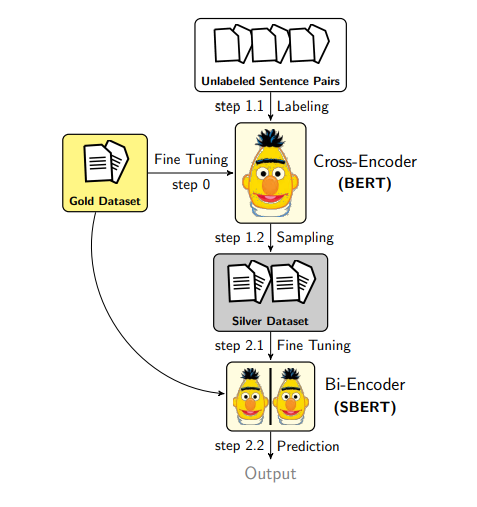
补充: 增强 SBERT
增强 SBERT 是一种用于收集数据以改善双向编码器的方法。预训练和微调双向编码器需要大量的数据,因此作者建议使用交叉编码器来标记大量输入对的集合,并将其添加到训练数据中。例如,如果你有非常少的标记数据,你可以训练一个交叉编码器,然后标记未标记的对,这可以用来训练一个双向编码器。
你是如何生成对的?我们可以使用句子的随机组合,然后使用交叉编码器对它们进行标记。这将导致大多数是负对,并倾斜标签分布。为了避免这种情况,作者探索了不同的技术:
- 使用 核密度估计 (KDE) ,目标是让小型的金数据集和增强数据集之间有类似的标签分布。这是通过放弃一些负对来实现的。当然,这将效率低下,因为你需要生成很多对才能得到几个正对。
- BM25 是一种基于重叠的搜索引擎算法 (例如,词频、文档长度等)。基于此,作者获取最相似的句子来检索最相似的 k 个句子,然后使用交叉编码器对它们进行标记。这是高效的,但只有在句子之间重叠很少时才能捕捉到语义相似性。
- 语义搜索采样 在金数据上训练双向编码器,然后用来采样其他相似的对。
- BM25 + 语义搜索采样 结合了前两种方法。这有助于找到词汇和语义上相似的句子。
在 Sentence Transformers 文档 中有很好的图表和示例脚本来做这件事。
总结
好了,我们刚才学会了怎么做一件很酷的事情: 检索和重新排序,这是句子嵌入的一个非常常见的任务。我们了解了双向编码器和交叉编码器有什么不同,以及什么时候该用哪一个。还学到了一些提升双向编码器性能的技巧,比如增强 SBERT。
别担心,代码可以随便改,随便玩!如果你觉得这篇博客不错,给个 赞或者分享 一下吧,这对我来说是个很大的鼓励!
知识检查
- 双向编码器和交叉编码器之间有什么区别?
- 解释重新排序的不同步骤。
- 如果使用双向编码器比较 30,000 个句子,我们需要生成多少个嵌入?使用交叉编码器进行推理需要运行多少次?
- 有哪些技术可以改善双向编码器?
现在,你已经有了实现你的搜索系统的坚实基础。作为一个后续任务,我建议使用不同的数据集实现一个类似的检索和重新排序系统。探索改变检索和重新排序模型对结果的影响。