简介
几个月前,我们介绍了 Informer 这个模型,相关论文 (Zhou, Haoyi, et al., 2021) 是一篇获得了 AAAI 2021 最佳论文奖的时间序列论文。我们也展示了一个使用 Informer 进行多变量概率预测的例子。在本文中,我们讨论以下问题: Transformer 模型对时间序列预测真的有效吗?我们给出的答案是,它们真的有效。
首先,我们将会提供一些实验证据,展示其真正的有效性。我们的对比实验将表明, DLinear 这个简单线性模型并没有像说的那样比 transformer 好。当我们在同等模型大小和相同设定的情况下对比时,我们发现基于 transformer 的模型在我们关注的测试标准上表现得更好。其次,我们将会介绍 Autoformer 模型,相关论文 (Wu, Haixu, et al., 2021) 在 Informer 模型问世后发表在 NeurIPS 2021 上。Autoformer 的模型现在已经可以在 ![]() Transformers 中 使用。最后,我们还会讨论 DLinear 模型,该模型是一个简单的前向网络,使用了 Autoformer 中的分解层 (decomposition layer)。DLinear 模型是在 Are Transformers Effective for Time Series Forecasting? 这篇论文中提出的,文中声称其性能在时间序列预测领域超越了 transformer 系列的算法。
Transformers 中 使用。最后,我们还会讨论 DLinear 模型,该模型是一个简单的前向网络,使用了 Autoformer 中的分解层 (decomposition layer)。DLinear 模型是在 Are Transformers Effective for Time Series Forecasting? 这篇论文中提出的,文中声称其性能在时间序列预测领域超越了 transformer 系列的算法。
下面我们开始!
评估 Transformer 系列模型 和 DLinear 模型
在 AAAI 2023 的论文 Are Transformers Effective for Time Series Forecasting? 中,作者声称 transformer 系列模型在时间序列预测方面并不有效。他们拿基于 transformer 的模型与一个简单的线性模型 DLinear 作对比。DLinear 使用了 Autoformer 中的 decomposition layer 结构 (下文将会介绍),作者声称其性能超越了基于 transformer 的模型。但事实真的是这样吗?我们接下来看看。
| Dataset | Autoformer (uni.) MASE | DLinear MASE |
|---|---|---|
Traffic |
0.910 | 0.965 |
Exchange-Rate |
1.087 | 1.690 |
Electricity |
0.751 | 0.831 |
上表展示了 Autoformer 和 DLinear 在三个论文中用到的数据集上的表现。结果说明 Autoformer 在三个数据集上表现都超越了 DLinear 模型。
接下来,我们将介绍 Autoformer 和 DLinear 模型,演示我们如何在上表 Traffic 数据集上对比它们的性能,并为结果提供一些可解释性。
先说结论: 一个简单的线性模型可能在某些特定情况下更有优势,但可能无法像 transformer 之类的复杂模型那样处理协方差信息。
Autoformer 详细介绍
Autoformer 基于传统的时间序列方法: 把时间序列分解为季节性 (seasonality) 以及趋势 - 周期 (trend-cycle) 这些要素。这通过加入分解层 ( Decomposition Layer ) 来实现,以此来增强模型获取这些信息的能力。此外,Autoformer 中还独创了自相关 (auto-correlation) 机制,替换掉了传统 transformer 中的自注意力 (self-attention)。该机制使得模型可以利用注意力机制中周期性的依赖,提升了总体性能。
下面,我们将深入探讨 Autoformer 的这两大主要贡献: 分解层 ( Decomposition Layer ) 和自相关机制 ( Autocorrelation Mechanism )。相关代码也会提供出来。
分解层
分解是一个时间序列领域十分常用的方法,但在 Autoformer 以前都没有被密集集成入深度学习模型中。我们先简单介绍这一概念,随后会使用 PyTorch 代码演示这一思路是如何应用到 Autoformer 中的。
时间序列分解
在时间序列分析中,分解 (decomposition) 是把一个时间序列拆分成三个系统性要素的方法: 趋势周期 (trend-cycle) 、季节性变动 (seasonal variation) 和随机波动 (random fluctuations)。趋势要素代表了时间序列的长期走势方向; 季节要素反映了一些反复出现的模式,例如以一年或一季度为周期出现的模式; 而随机 (无规律) 因素则反映了数据中无法被上述两种要素解释的随机噪声。
有两种主流的分解方法: 加法分解和乘法分解,这在 statsmodels 这个库里都有实现。通过分解时间序列到这三个要素,我们能更好地理解和建模数据中潜在的模式。
但怎样把分解集成进 transformer 结构呢?我们可以参考参考 Autoformer 的做法。
Autoformer 中的分解
 |
|---|
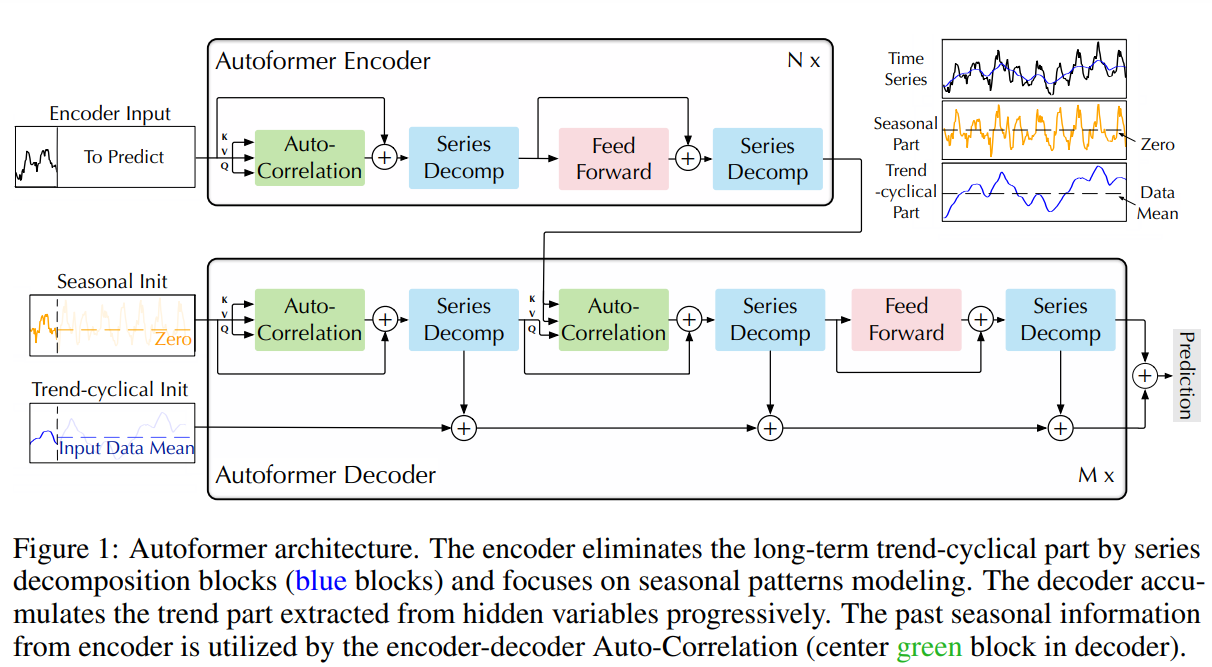
| Autoformer 结构 (来自论文) |
Autoformer 把分解作为一个内部计算操作集成到模型中,如上图所示。可以看到,编码器和解码器都使用了分解模块来集合 trend-cyclical 信息,并从序列中渐进地提取 seasonal 信息。这种内部分解的概念已经从 Autoformer 中展示了其有效性。所以很多其它的时间序列论文也开始采用这一方法,例如 FEDformer (Zhou, Tian, et al., ICML 2022) 和 DLinear (Zeng, Ailing, et al., AAAI 2023),这更说明了其在时间序列建模中的意义。
现在,我们正式地给分解层做出定义:
对一个长度为 L 的序列 $\mathcal{X} \in \mathbb{R}^{L \times d},分解层返回的 \mathcal{X}\textrm{trend} 和 \mathcal{X}\textrm{seasonal}$ 定义如下:
对应的 PyTorch 代码实现是:
import torch
from torch import nn

class DecompositionLayer(nn.Module):
    """
    Returns the trend and the seasonal parts of the time series.
    """

    def __init__(self, kernel_size):
        super().__init__()
        self.kernel_size = kernel_size
        self.avg = nn.AvgPool1d(kernel_size=kernel_size, stride=1, padding=0) # moving average

    def forward(self, x):
        """Input shape: Batch x Time x EMBED_DIM"""
        # padding on the both ends of time series
        num_of_pads = (self.kernel_size - 1) // 2
        front = x[:, 0:1, :].repeat(1, num_of_pads, 1)
        end = x[:, -1:, :].repeat(1, num_of_pads, 1)
        x_padded = torch.cat([front, x, end], dim=1)

        # calculate the trend and seasonal part of the series
        x_trend = self.avg(x_padded.permute(0, 2, 1)).permute(0, 2, 1)
        x_seasonal = x - x_trend
        return x_seasonal, x_trend
可见,代码非常简单,可以很方便地用在其它模型中,正如 DLinear 那样。下面,我们讲解第二个创新点: 注意力 (自相关) 机制 。
注意力 (自相关) 机制
 |
|---|
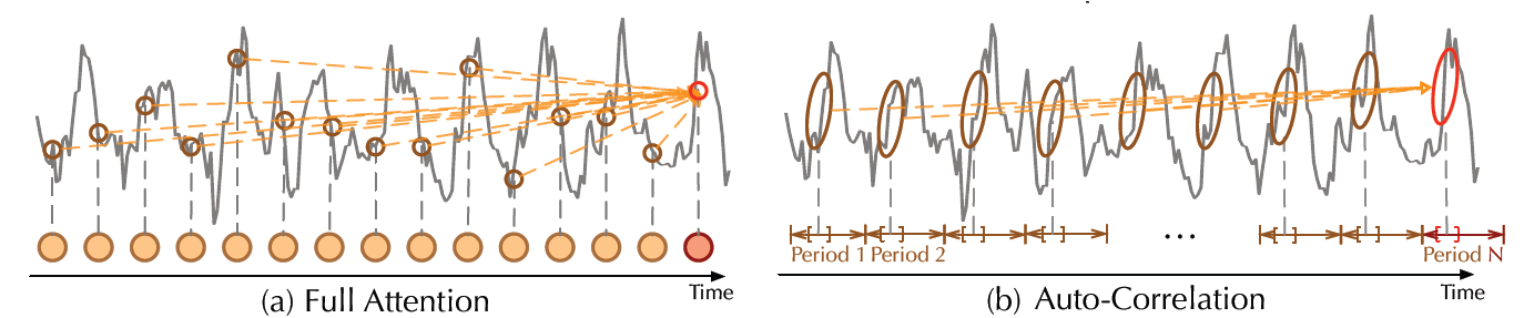
| 最原始的注意力机制和自相关机制 (图片来自论文) |
除了分解层之外,Autoformer 还使用了一个原创的自相关 (autocorrelation) 机制,可以完美替换自注意力 (self-attention) 机制。在 最原始的时间序列 transformer 模型 中,注意力权重是在时域计算并逐点聚合的。而从上图中可以看出,Autoformer 不同的是它在频域计算这些 (使用 快速傅立叶变换),然后通过时延聚合它们。
接下来部分,我们深入细节,并使用代码作出讲解。
时域的注意力机制
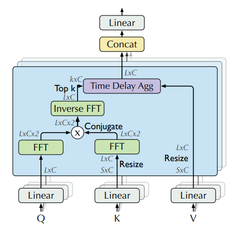 |
|---|
| 借助 FFT 在频域计算注意力权重 (图片来自论文) |
理论上讲,给定一个时间延迟 $\tau$,一个离散变量的 自相关性 y 可以用来衡量这个变量当前时刻 t 的值和过去时刻 t-\tau 的值之间的“关系”(皮尔逊相关性,pearson correlation):
使用自相关性,Autoformer 提取了 query 和 key 之间基于频域的相互依赖,而不是像之前那样两两之间的点乘。可以把这个操作看成是自注意力中 QK^T 的替换。
实际操作中,query 和 key 之间的自相关是通过 FFT 一次性针对 所有时间延迟 计算出来的。通过这种方法,自相关机制达到了 O(L \log L) 的时间复杂度 ( L 是输入时间长度),这个速度和 Informer 的 ProbSparse attention 接近。值得一提的是,使用 FFT 计算自相关性的理论基础是 Wiener–Khinchin theorem,这里我们不细讲了。
现在,我们来看看相应的 PyTorch 代码:
import torch

def autocorrelation(query_states, key_states):
    """
    Computes autocorrelation(Q,K) using `torch.fft`.
    Think about it as a replacement for the QK^T in the self-attention.

    Assumption: states are resized to same shape of [batch_size, time_length, embedding_dim].
    """
    query_states_fft = torch.fft.rfft(query_states, dim=1)
    key_states_fft = torch.fft.rfft(key_states, dim=1)
    attn_weights = query_states_fft * torch.conj(key_states_fft)
    attn_weights = torch.fft.irfft(attn_weights, dim=1)

    return attn_weights
代码非常简洁!![]() 请注意这只是
请注意这只是 autocorrelation(Q,K) 的部分实现,完整实现请参考 ![]() Transformers 中的代码。
Transformers 中的代码。
接下来,我们将看到如何使用时延值聚合我们的 attn_weights ,这个过程被称为时延聚合 ( Time Delay Aggregation )。
时延聚合
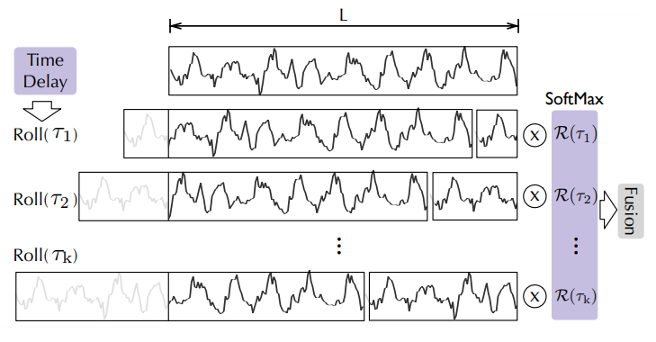 |
|---|
| 通过时延来聚合,图片来自 Autoformer 论文 |
我们用 \mathcal{R_{Q,K}} 来表示自相关 (即 attn_weights )。那么问题是: 我们应该如何聚合这些 \mathcal{R_{Q,K}}(\tau_1), \mathcal{R_{Q,K}}(\tau_2), …, \mathcal{R_{Q,K}}(\tau_k) 到 \mathcal{V} 上面?在标准的自注意力机制中,这种聚合通过点乘完成。但在 Autoformer 中,我们使用了一种不同的方法。首先我们在时延 \tau_1, \tau_2, … \tau_k 上对齐 $\mathcal{V},计算在这些时延下它对应的值,这个操作叫作 _Rolling_ 。接下来,我们将对齐的 \mathcal{V} 和自相关的值进行逐点的乘法运算。在上图中,你可以看到在左边是基于时延对 \mathcal{V}$ 进行的 Rolling 操作; 而右边就展示了与自相关进行的逐点乘法。
整个过程可以用以下公式总结:
就是这样!需要注意的是,$k$ 是一个超参数,我们称之为 autocorrelation_factor (类似于 Informer 里的 sampling_factor ) ; 而 softmax 是在乘法操作之前运用到自相关上面的。
现在,我们已经可以看看最终的代码了:
import torch
import math

def time_delay_aggregation(attn_weights, value_states, autocorrelation_factor=2):
    """
    Computes aggregation as value_states.roll(delay)* top_k_autocorrelations(delay).
    The final result is the autocorrelation-attention output.
    Think about it as a replacement of the dot-product between attn_weights and value states.

    The autocorrelation_factor is used to find top k autocorrelations delays.
    Assumption: value_states and attn_weights shape: [batch_size, time_length, embedding_dim]
    """
    bsz, num_heads, tgt_len, channel = ...
    time_length = value_states.size(1)
    autocorrelations = attn_weights.view(bsz, num_heads, tgt_len, channel)

    # find top k autocorrelations delays
    top_k = int(autocorrelation_factor * math.log(time_length))
    autocorrelations_mean = torch.mean(autocorrelations, dim=(1, -1)) # bsz x tgt_len
    top_k_autocorrelations, top_k_delays = torch.topk(autocorrelations_mean, top_k, dim=1)

    # apply softmax on the channel dim
    top_k_autocorrelations = torch.softmax(top_k_autocorrelations, dim=-1) # bsz x top_k

    # compute aggregation: value_states.roll(delay)* top_k_autocorrelations(delay)
    delays_agg = torch.zeros_like(value_states).float() # bsz x time_length x channel
    for i in range(top_k):
        value_states_roll_delay = value_states.roll(shifts=-int(top_k_delays[i]), dims=1)
        top_k_at_delay = top_k_autocorrelations[:, i]
        # aggregation
        top_k_resized = top_k_at_delay.view(-1, 1, 1).repeat(num_heads, tgt_len, channel)
        delays_agg += value_states_roll_delay * top_k_resized

    attn_output = delays_agg.contiguous()
    return attn_output
完成!Autoformer 模型现在已经可以在 ![]() Transformers 中 使用 了,名字就叫
Transformers 中 使用 了,名字就叫 AutoformerModel 。
针对这个模型,我们要对比单变量 transformer 模型与 DLinear 的性能,DLinear 本质也是单变量的。后面我们也会展示两个多变量 transformer 模型的性能 (在同一数据上训练的)。
DLinear 详细介绍
实际上,DLinear 结构非常简单,仅仅是从 Autoformer 的 DecompositionLayer 上连接全连接层。它使用 DecompositionLayer 来分解输入的世界序列到残差部分 (季节性) 和趋势部分。前向过程中,每个部分都被输入到各自的线性层,并被映射成 prediction_length 长度的输出。最终的输出就是两个输入的和:
def forward(self, context):
    seasonal, trend = self.decomposition(context)
    seasonal_output = self.linear_seasonal(seasonal)
    trend_output = self.linear_trend(trend)
    return seasonal_output + trend_output
在这种设定下,首先我们把输入的序列映射成 prediction-length * hidden 维度 (通过 linear_seasonal 和 linear_trend 两个层) ; 得到的结果会被相加起来,并转换为 (prediction_length, hidden) 形状; 最后,维度为 hidden 的隐性表征会被映射到某种分布的参数上。
在我们的测评中,我们使用 GluonTS 中 DLinear 的实现。
示例: Traffic 数据集
我们希望用实验结果展示库中基于 transformer 模型的性能,这里我们使用 Traffic 数据集,该数据集有 862 条时间序列数据。我们将在每条时间序列上训练一个共享的模型 (单变量设定)。每个时间序列都代表了一个传感器的占有率值,值的范围在 0 到 1 之间。下面的这些超参数我们将在所有模型中保持一致。
# Traffic prediction_length is 24. Reference:
# https://github.com/awslabs/gluonts/blob/6605ab1278b6bf92d5e47343efcf0d22bc50b2ec/src/gluonts/dataset/repository/_lstnet.py#L105

prediction_length = 24
context_length = prediction_length*2
batch_size = 128
num_batches_per_epoch = 100
epochs = 50
scaling = "std"
使用的 transformer 模型都很小:
encoder_layers=2
decoder_layers=2
d_model=16
这里我们不再讲解如何用 Autoformer 训练模型,读者可以参考之前两篇博客 (TimeSeriesTransformer 和 Informer) 并替换模型为 Autoformer 、替换数据集为 traffic 。我们也训练了现成的模型放在 HuggingFace Hub 上,稍后的评测将会使用这里的模型。
载入数据集
首先安装必要的库:
!pip install -q transformers datasets evaluate accelerate "gluonts[torch]" ujson tqdm
traffic 数据集 (Lai et al. (2017)) 包含了旧金山的交通数据。它包含 862 条以小时为时间单位的时间序列,代表了道路占有率的数值,其数值范围为 $[0, 1]$,记录了旧金山湾区高速公路从 2015 年到 2016 年的数据。
from gluonts.dataset.repository.datasets import get_dataset

dataset = get_dataset("traffic")
freq = dataset.metadata.freq
prediction_length = dataset.metadata.prediction_length
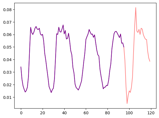
我们可视化一条时间序列看看,并画出训练和测试集的划分:
import matplotlib.pyplot as plt

train_example = next(iter(dataset.train))
test_example = next(iter(dataset.test))

num_of_samples = 4*prediction_length

figure, axes = plt.subplots()
axes.plot(train_example["target"][-num_of_samples:], color="blue")
axes.plot(
    test_example["target"][-num_of_samples - prediction_length :],
    color="red",
    alpha=0.5,
)

plt.show()
定义训练和测试集划分:
train_dataset = dataset.train
test_dataset = dataset.test
定义数据变换
接下来,我们定义数据的变换,尤其是时间相关特征的制作 (基于数据集本身和一些普适做法)。
我们定义一个 Chain ,代表 GluonTS 中一系列的变换 (这类似图像里 torchvision.transforms.Compose )。这让我们将一系列变换集成到一个处理流水线中。
下面代码中,每个变换都添加了注释,用以说明它们的作用。从更高层次讲,我们将遍历每一个时间序列,并添加或删除一些特征:
from transformers import PretrainedConfig
from gluonts.time_feature import time_features_from_frequency_str

from gluonts.dataset.field_names import FieldName
from gluonts.transform import (
    AddAgeFeature,
    AddObservedValuesIndicator,
    AddTimeFeatures,
    AsNumpyArray,
    Chain,
    ExpectedNumInstanceSampler,
    RemoveFields,
    SelectFields,
    SetField,
    TestSplitSampler,
    Transformation,
    ValidationSplitSampler,
    VstackFeatures,
    RenameFields,
)

def create_transformation(freq: str, config: PretrainedConfig) -> Transformation:
    # create a list of fields to remove later
    remove_field_names = []
    if config.num_static_real_features == 0:
        remove_field_names.append(FieldName.FEAT_STATIC_REAL)
    if config.num_dynamic_real_features == 0:
        remove_field_names.append(FieldName.FEAT_DYNAMIC_REAL)
    if config.num_static_categorical_features == 0:
        remove_field_names.append(FieldName.FEAT_STATIC_CAT)

    return Chain(
        # step 1: remove static/dynamic fields if not specified
        [RemoveFields(field_names=remove_field_names)]
        # step 2: convert the data to NumPy (potentially not needed)
        + (
            [
                AsNumpyArray(
                    field=FieldName.FEAT_STATIC_CAT,
                    expected_ndim=1,
                    dtype=int,
                )
            ]
            if config.num_static_categorical_features > 0
            else []
        )
        + (
            [
                AsNumpyArray(
                    field=FieldName.FEAT_STATIC_REAL,
                    expected_ndim=1,
                )
            ]
            if config.num_static_real_features > 0
            else []
        )
        + [
            AsNumpyArray(
                field=FieldName.TARGET,
                # we expect an extra dim for the multivariate case:
                expected_ndim=1 if config.input_size == 1 else 2,
            ),
            # step 3: handle the NaN's by filling in the target with zero
            # and return the mask (which is in the observed values)
            # true for observed values, false for nan's
            # the decoder uses this mask (no loss is incurred for unobserved values)
            # see loss_weights inside the xxxForPrediction model
            AddObservedValuesIndicator(
                target_field=FieldName.TARGET,
                output_field=FieldName.OBSERVED_VALUES,
            ),
            # step 4: add temporal features based on freq of the dataset
            # these serve as positional encodings
            AddTimeFeatures(
                start_field=FieldName.START,
                target_field=FieldName.TARGET,
                output_field=FieldName.FEAT_TIME,
                time_features=time_features_from_frequency_str(freq),
                pred_length=config.prediction_length,
            ),
            # step 5: add another temporal feature (just a single number)
            # tells the model where in the life the value of the time series is
            # sort of running counter
            AddAgeFeature(
                target_field=FieldName.TARGET,
                output_field=FieldName.FEAT_AGE,
                pred_length=config.prediction_length,
                log_scale=True,
            ),
            # step 6: vertically stack all the temporal features into the key FEAT_TIME
            VstackFeatures(
                output_field=FieldName.FEAT_TIME,
                input_fields=[FieldName.FEAT_TIME, FieldName.FEAT_AGE]
                + (
                    [FieldName.FEAT_DYNAMIC_REAL]
                    if config.num_dynamic_real_features > 0
                    else []
                ),
            ),
            # step 7: rename to match HuggingFace names
            RenameFields(
                mapping={
                    FieldName.FEAT_STATIC_CAT: "static_categorical_features",
                    FieldName.FEAT_STATIC_REAL: "static_real_features",
                    FieldName.FEAT_TIME: "time_features",
                    FieldName.TARGET: "values",
                    FieldName.OBSERVED_VALUES: "observed_mask",
                }
            ),
        ]
    )
定义 InstanceSplitter
我们需要创建一个 InstanceSplitter ,用来给训练、验证和测试集提供采样窗口,得到一段时间的内的时间序列 (我们不可能把完整的整段数据输入给模型,毕竟时间太长,而且也有内存限制)。
这个实例分割工具每一次将会随机选取 context_length 长度的数据,以及紧随其后的 prediction_length 长度的窗口,并为相应的窗口标注 past_ 或 future_ 。这样可以保证 values 能被分为 past_values 和随后的 future_values ,各自作为编码器和解码器的输入。除了 values ,对于 time_series_fields 中的其它 key 对应的数据也是一样。
from gluonts.transform import InstanceSplitter
from gluonts.transform.sampler import InstanceSampler
from typing import Optional

def create_instance_splitter(
    config: PretrainedConfig,
    mode: str,
    train_sampler: Optional[InstanceSampler] = None,
    validation_sampler: Optional[InstanceSampler] = None,
) -> Transformation:
    assert mode in ["train", "validation", "test"]

    instance_sampler = {
        "train": train_sampler
        or ExpectedNumInstanceSampler(
            num_instances=1.0, min_future=config.prediction_length
        ),
        "validation": validation_sampler
        or ValidationSplitSampler(min_future=config.prediction_length),
        "test": TestSplitSampler(),
    }[mode]

    return InstanceSplitter(
        target_field="values",
        is_pad_field=FieldName.IS_PAD,
        start_field=FieldName.START,
        forecast_start_field=FieldName.FORECAST_START,
        instance_sampler=instance_sampler,
        past_length=config.context_length + max(config.lags_sequence),
        future_length=config.prediction_length,
        time_series_fields=["time_features", "observed_mask"],
    )
创建 PyTorch 的 DataLoader
接下来就该创建 PyTorch DataLoader 了: 这让我们能把数据整理成 batch 的形式,即 (input, output) 对的形式,或者说是 ( past_values , future_values ) 的形式。
from typing import Iterable

import torch
from gluonts.itertools import Cyclic, Cached
from gluonts.dataset.loader import as_stacked_batches

def create_train_dataloader(
    config: PretrainedConfig,
    freq,
    data,
    batch_size: int,
    num_batches_per_epoch: int,
    shuffle_buffer_length: Optional[int] = None,
    cache_data: bool = True,
 **kwargs,
) -> Iterable:
    PREDICTION_INPUT_NAMES = [
        "past_time_features",
        "past_values",
        "past_observed_mask",
        "future_time_features",
    ]
    if config.num_static_categorical_features > 0:
        PREDICTION_INPUT_NAMES.append("static_categorical_features")

    if config.num_static_real_features > 0:
        PREDICTION_INPUT_NAMES.append("static_real_features")

    TRAINING_INPUT_NAMES = PREDICTION_INPUT_NAMES + [
        "future_values",
        "future_observed_mask",
    ]

    transformation = create_transformation(freq, config)
    transformed_data = transformation.apply(data, is_train=True)
    if cache_data:
        transformed_data = Cached(transformed_data)

    # we initialize a Training instance
    instance_splitter = create_instance_splitter(config, "train")

    # the instance splitter will sample a window of
    # context length + lags + prediction length (from the 366 possible transformed time series)
    # randomly from within the target time series and return an iterator.
    stream = Cyclic(transformed_data).stream()
    training_instances = instance_splitter.apply(stream, is_train=True)

    return as_stacked_batches(
        training_instances,
        batch_size=batch_size,
        shuffle_buffer_length=shuffle_buffer_length,
        field_names=TRAINING_INPUT_NAMES,
        output_type=torch.tensor,
        num_batches_per_epoch=num_batches_per_epoch,
    )

def create_test_dataloader(
    config: PretrainedConfig,
    freq,
    data,
    batch_size: int,
 **kwargs,
):
    PREDICTION_INPUT_NAMES = [
        "past_time_features",
        "past_values",
        "past_observed_mask",
        "future_time_features",
    ]
    if config.num_static_categorical_features > 0:
        PREDICTION_INPUT_NAMES.append("static_categorical_features")

    if config.num_static_real_features > 0:
        PREDICTION_INPUT_NAMES.append("static_real_features")

    transformation = create_transformation(freq, config)
    transformed_data = transformation.apply(data, is_train=False)

    # we create a Test Instance splitter which will sample the very last
    # context window seen during training only for the encoder.
    instance_sampler = create_instance_splitter(config, "test")

    # we apply the transformations in test mode
    testing_instances = instance_sampler.apply(transformed_data, is_train=False)

    return as_stacked_batches(
        testing_instances,
        batch_size=batch_size,
        output_type=torch.tensor,
        field_names=PREDICTION_INPUT_NAMES,
    )
在 Autoformer 上评测
我们已经在这个数据集上预训练了一个 Autoformer 了,所以我们可以直接拿来模型在测试集上测一下:
from transformers import AutoformerConfig, AutoformerForPrediction

config = AutoformerConfig.from_pretrained("kashif/autoformer-traffic-hourly")
model = AutoformerForPrediction.from_pretrained("kashif/autoformer-traffic-hourly")

test_dataloader = create_test_dataloader(
    config=config,
    freq=freq,
    data=test_dataset,
    batch_size=64,
)
在推理时,我们使用模型的 generate() 方法来预测 prediction_length 步的未来数据,基于最近使用的对应时间序列的窗口长度。
from accelerate import Accelerator

accelerator = Accelerator()
device = accelerator.device
model.to(device)
model.eval()

forecasts_ = []
for batch in test_dataloader:
    outputs = model.generate(
        static_categorical_features=batch["static_categorical_features"].to(device)
        if config.num_static_categorical_features > 0
        else None,
        static_real_features=batch["static_real_features"].to(device)
        if config.num_static_real_features > 0
        else None,
        past_time_features=batch["past_time_features"].to(device),
        past_values=batch["past_values"].to(device),
        future_time_features=batch["future_time_features"].to(device),
        past_observed_mask=batch["past_observed_mask"].to(device),
    )
    forecasts_.append(outputs.sequences.cpu().numpy())
模型输出的数据形状是 ( batch_size , number of samples , prediction length , input_size )。
在下面这个例子中,我们为预测接下来 24 小时的交通数据而得到了 100 条可能的数值,而 batch size 是 64:
forecasts_[0].shape

>>> (64, 100, 24)
我们在垂直方向把它们堆叠起来 (使用 numpy.vstack 函数),以此获取所有测试集时间序列的预测: 我们有 7 个滚动的窗口,所以有 7 * 862 = 6034 个预测。
import numpy as np

forecasts = np.vstack(forecasts_)
print(forecasts.shape)

>>> (6034, 100, 24)
我们可以把预测结果和 ground truth 做个对比。为此,我们使用 ![]() Evaluate 这个库,它里面包含了 MASE 的度量方法。
Evaluate 这个库,它里面包含了 MASE 的度量方法。
我们对每个时间序列用这一度量标准计算相应的值,并算出其平均值:
from tqdm.autonotebook import tqdm
from evaluate import load
from gluonts.time_feature import get_seasonality

mase_metric = load("evaluate-metric/mase")

forecast_median = np.median(forecasts, 1)

mase_metrics = []
for item_id, ts in enumerate(tqdm(test_dataset)):
    training_data = ts["target"][:-prediction_length]
    ground_truth = ts["target"][-prediction_length:]
    mase = mase_metric.compute(
        predictions=forecast_median[item_id],
        references=np.array(ground_truth),
        training=np.array(training_data),
        periodicity=get_seasonality(freq))
    mase_metrics.append(mase["mase"])
所以 Autoformer 模型的结果是:
print(f"Autoformer univariate MASE: {np.mean(mase_metrics):.3f}")

>>> Autoformer univariate MASE: 0.910
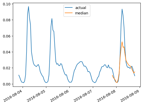
我们还可以画出任意时间序列预测针对其 ground truth 的对比,这需要以下函数:
import matplotlib.dates as mdates
import pandas as pd

test_ds = list(test_dataset)

def plot(ts_index):
    fig, ax = plt.subplots()

    index = pd.period_range(
        start=test_ds[ts_index][FieldName.START],
        periods=len(test_ds[ts_index][FieldName.TARGET]),
        freq=test_ds[ts_index][FieldName.START].freq,
    ).to_timestamp()

    ax.plot(
        index[-5*prediction_length:],
        test_ds[ts_index]["target"][-5*prediction_length:],
        label="actual",
    )

    plt.plot(
        index[-prediction_length:],
        np.median(forecasts[ts_index], axis=0),
        label="median",
    )

    plt.gcf().autofmt_xdate()
    plt.legend(loc="best")
    plt.show()
比如,测试集中第四个时间序列的结果对比,画出来是这样:
plot(4)
在 DLinear 上评测
gluonts 提供了一种 DLinear 的实现,我们将使用这个实现区训练、测评该算法:
from gluonts.torch.model.d_linear.estimator import DLinearEstimator

# Define the DLinear model with the same parameters as the Autoformer model
estimator = DLinearEstimator(
    prediction_length=dataset.metadata.prediction_length,
    context_length=dataset.metadata.prediction_length*2,
    scaling=scaling,
    hidden_dimension=2,

    batch_size=batch_size,
    num_batches_per_epoch=num_batches_per_epoch,
    trainer_kwargs=dict(max_epochs=epochs)
)
训练模型:
predictor = estimator.train(
    training_data=train_dataset,
    cache_data=True,
    shuffle_buffer_length=1024
)

>>> INFO:pytorch_lightning.callbacks.model_summary:
      | Name  | Type         | Params
    ---------------------------------------
    0 | model | DLinearModel | 4.7 K
    ---------------------------------------
    4.7 K     Trainable params
    0 Non-trainable params
    4.7 K     Total params
    0.019 Total estimated model params size (MB)

    Training: 0it [00:00, ?it/s]
    ...
    INFO:pytorch_lightning.utilities.rank_zero:Epoch 49, global step 5000: 'train_loss' was not in top 1
    INFO:pytorch_lightning.utilities.rank_zero:`Trainer.fit` stopped: `max_epochs=50` reached.
在测试集上评测:
from gluonts.evaluation import make_evaluation_predictions, Evaluator

forecast_it, ts_it = make_evaluation_predictions(
    dataset=dataset.test,
    predictor=predictor,
)

d_linear_forecasts = list(forecast_it)
d_linear_tss = list(ts_it)

evaluator = Evaluator()

agg_metrics, _ = evaluator(iter(d_linear_tss), iter(d_linear_forecasts))
所以 DLinear 对应的结果是:
dlinear_mase = agg_metrics["MASE"]
print(f"DLinear MASE: {dlinear_mase:.3f}")

>>> DLinear MASE: 0.965
同样地,我们画出预测结果与 ground truth 的对比曲线图:
def plot_gluonts(index):
    plt.plot(d_linear_tss[index][-4 * dataset.metadata.prediction_length:].to_timestamp(), label="target")
    d_linear_forecasts[index].plot(show_label=True, color='g')
    plt.legend()
    plt.gcf().autofmt_xdate()
    plt.show()
plot_gluonts(4)
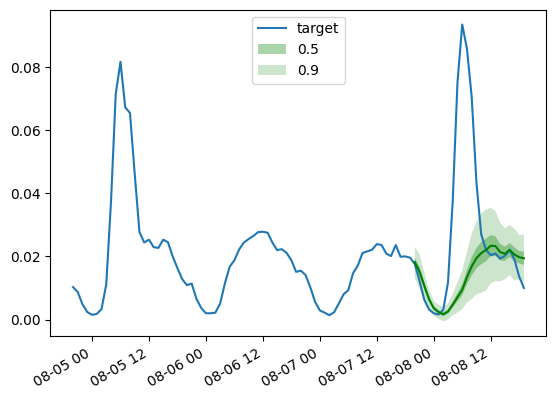
实际上, traffic 数据集在平日和周末会出现传感器中模式的分布偏移。那我们还应该怎么做呢?由于 DLinear 没有足够的能力去处理协方差信息,或者说是任何的日期时间的特征,我们给出的窗口大小无法覆盖全面,使得让模型有足够信息去知道当前是在预测平日数据还是周末数据。因此模型只会去预测更为普适的结果,这就导致其预测分布偏向平日数据,因而导致对周末数据的预测变得更差。当然,如果我们给一个足够大的窗口,一个线性模型也可以识别出周末的模式,但当我们的数据中存在以月或以季度为单位的模式分布时,那就需要更大的窗口了。
总结
所以 transformer 模型和线性模型对比的结论是什么呢?不同模型在测试集上的 MASE 指标如下所示:
| Dataset | Transformer (uni.) | Transformer (mv.) | Informer (uni.) | Informer (mv.) | Autoformer (uni.) | DLinear |
|---|---|---|---|---|---|---|
Traffic |
0.876 | 1.046 | 0.924 | 1.131 | 0.910 | 0.965 |
可以看到,我们去年引入的 最原始的 Transformer 模型 获得了最好的性能指标。其次,多变量模型一般都比对应的单变量模型更差,原因在于序列间的相关性关系一般都较难预测。额外添加的波动通常会损坏预测结果,或者模型可能会学到一些错误的相关性信息。最近的一些论文,如 CrossFormer (ICLR 23) 和 CARD 也在尝试解决这些 transformer 模型中的问题。
多变量模型通常在训练数据足够大的时候才会表现得好。但当我们与单变量模型在小的公开数据集上对比时,通常单变量模型会表现得更好。相对于线性模型,通常其相应尺寸的单变量 transformer 模型或其它神经网络类模型会表现得更好。
总结来讲,transformer 模型在时间序列预测领域,远没有达到要被淘汰的境地。
然而大规模训练数据对它巨大潜力的挖掘是至关重要的,这一点不像 CV 或 NLP 领域,时间序列预测缺乏大规模公开数据集。
当前绝大多数的时间序列预训练模型也不过是在诸如 UCR & UEA 这样的少量样本上训练的。
即使这些基准数据集为时间序列预测的发展进步提供了基石,其较小的规模和泛化性的缺失使得大规模预训练仍然面临诸多困难。
所以对于时间序列预测领域来讲,发展大规模、强泛化性的数据集 (就像 CV 领域的 ImageNet 一样) 是当前最重要的事情。这将会极大地促进时间序列分析领域与训练模型的发展研究,提升与训练模型在时间序列预测方面的能力。
声明
我们诚挚感谢 Lysandre Debut 和 Pedro Cuenca 提供的深刻见解和对本项目的帮助。 ![]()
英文原文: Yes, Transformers are Effective for Time Series Forecasting (+ Autoformer)
作者: Eli Simhayev, Kashif Rasul, Niels Rogge
译者: Hoi2022
审校/排版: zhongdongy (阿东)