在这篇博客中,我们将通过一个端到端的示例来讲解 Transformer 模型中的数学原理。我们的目标是对模型的工作原理有一个良好的理解。为了使内容易于理解,我们会进行大量简化。我们将减少模型的维度,以便我们可以手动推理模型的计算过程。例如,我们将使用 4 维的嵌入向量代替原始的 512 维嵌入向量。这样做可以更容易手动推理数学计算过程!我们将使用随机的向量和矩阵初始化,但如果你想一起动手试一试的话,你也可以使用自己的值。
如你所见,这些数学原理并不复杂。复杂性来自于步骤的数量和参数的数量。我建议你在阅读本博文之前阅读 (或一起对照阅读)图解 Transform (The Illustrated Transformer) 这篇博客。这篇博客使用图解非常直观地解释了 Transformer 模型,我不打算再重复解释那里已经解释过的内容。我的目标是解释 Transformer 模型的“how”,而不是“what”。如果你想深入了解,可以查阅著名的原始论文: Attention is all you need 。
预备知识
需要基本的线性代数基础知识——我们主要进行简单的矩阵乘法,所以不需要非常精通。除此之外,对机器学习和深度学习的基本理解也会对理解本文有帮助。
本文内容
- 通过一个端到端的示例来讲解 Transformer 模型在推理过程中的数学原理
- 解释注意力机制
- 解释残差连接和层归一化
- 提供一些代码来扩展模型!
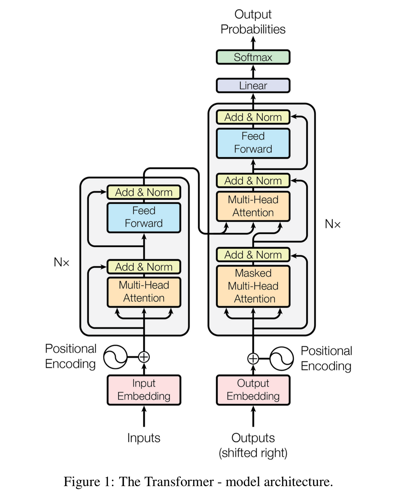
言归正传,让我们开始吧!原始的 Transformer 模型由编码器和解码器两部分组成。我们的目标是将使用 Transform 模型制作一个翻译器!我们首先将重点放在编码器部分。
编码器
编码器的目标是生成输入文本的丰富嵌入表示。这个嵌入将捕捉输入的语义信息,并传递给解码器生成输出文本。编码器由 N 层堆叠而成。在我们深入了解这些层之前,我们需要了解如何将单词 (或 token ) 传递给模型。
说明
嵌入 (Embeddings) 是一个有点过度使用的术语。我们首先创建一个文本的嵌入,它将作为编码器的输入。编码器还会输出一个嵌入 (有时也称为隐藏状态)。解码器也会接收一个嵌入!嵌入的整个目的是将单词 (或 token ) 表示为向量。
1. 文本嵌入
假设我们想将英文的“Hello World”翻译成西班牙语。第一步是使用文本嵌入算法将每个输入 token 转换为向量。文本嵌入算法的编码方式是通过大量文本学习到的。通常我们使用比较大的向量大小,比如 512,这样可以有更加丰富的语义表示能力;但为了方便起见,我们在这个例子中使用大小为 4 的向量。这样我们可以更容易地进行数学计算。
Hello → [1,2,3,4]
World → [2,3,4,5]
这样我们就可以将输入表示为一个矩阵。
说明
虽然我们可以使用单独的两个向量表示 Hello World 的文本嵌入,但将它们作为单个矩阵管理会更容易。这是因为我们可以使用矩阵乘法简化运算!
2. 位置编码
同一单词出现在句子的不同位置可能会表示不同的语义,上述的文本嵌入没有表示单词在句子中位置的信息,所以我们还需要使用一些方法表示一些位置信息。可以通过在文本嵌入中添加位置编码来实现这一点。提供单词在句子中的位置编码有很多种方法——我们可以使用学习到的位置嵌入或固定的向量来表示。原始论文使用了固定的向量,因为他们发现两种方法几乎没有区别 (参见原始论文的 3.5 节)。我们也将使用固定的向量。正弦和余弦函数具有波状模式,并且随着长度的推移重复出现。通过使用这些函数,句子中的每个位置都会得到一组独特但一致的数字编码表示。下面是论文中使用的函数 (第 3.5 节),其中 pos 表示输入序列中的位置,$i$ 表示编码向量的维度索引,$d_{\text{model}}$ 表示模型的维度:
这个想法是对文本嵌入中的每个值进行正弦和余弦之间的插值 (偶数索引使用正弦,奇数索引使用余弦)。让我们使用之前“Hello World”的例子,使用维度为 4 的位置编码计算一下!
“Hello”是“Hello World”的第一个字符,$pos=0$ 其位置编码如下:
- i = 0(偶数): PE(0,0) = sin(0 / 10000^(0 / 4)) = sin(0) = 0
- i = 1(奇数): PE(0,1) = cos(0 / 10000^(2*1 / 4)) = cos(0) = 1
- i = 2(偶数): PE(0,2) = sin(0 / 10000^(2*2 / 4)) = sin(0) = 0
- i = 3(奇数): PE(0,3) = cos(0 / 10000^(2*3 / 4)) = cos(0) = 1
“World”是“Hello World”的第二个字符,$pos=1$ 其位置编码如下:
- i = 0(偶数): PE(1,0) = sin(1 / 10000^(0 / 4)) = sin(1 / 10000^0) = sin(1) ≈ 0.84
- i = 1(奇数): PE(1,1) = cos(1 / 10000^(2*1 / 4)) = cos(1 / 10000^0.5) ≈ cos(0.01) ≈ 0.99
- i = 2(偶数): PE(1,2) = sin(1 / 10000^(2*2 / 4)) = sin(1 / 10000^1) ≈ 0
- i = 3(奇数): PE(1,3) = cos(1 / 10000^(2*3 / 4)) = cos(1 / 10000^1.5) ≈ 1
所以总结一下
- “Hello” → [0, 1, 0, 1]
- “World” → [0.84, 0.99, 0, 1]
注意,位置编码的维度需要与文本嵌入的维度相同。
3. 将位置编码加入文本嵌入
现在我们将位置编码添加到文本嵌入中。通过将这两个向量相加来实现。
“Hello” = [1,2,3,4] + [0, 1, 0, 1] = [1, 3, 3, 5]
“World” = [2,3,4,5] + [0.84, 0.99, 0, 1] = [2.84, 3.99, 4, 6]
所以我们的新矩阵,也就是编码器的输入,现在是:
如果你之前看到过原始论文中的图片,我们刚刚完成的是图片的左下部分 (嵌入 + 位置编码)。
4. 自注意力
4.1 矩阵定义
我们现在介绍多头注意力 (Multi-head Attention) 的概念。注意力是一种机制,模型可以通过这种机制来控制输入的不同部分的重要程度。多头注意力指的是通过使用多个注意力头使模型能够同时关注来自不同表示子空间信息的方法。每个注意力头都有自己的 K、V 和 Q 矩阵。通过将多个注意力头的输出合并在一起,模型可以综合考虑来自不同注意力头的信息,从而获得更全局的理解和表达能力。
我们在示例中使用 2 个注意力头。每个注意力头最开始将使用随机初始化的值代替。每个矩阵是一个 4x3 的矩阵。这样,每个矩阵可以把 4 维嵌入转换为 3 维的键矩阵 (K)、值矩阵 (K) 和查询矩阵 (Q)。这降低了注意力机制的维度,有助于降低计算复杂性。注意,使用过小的注意力大小会影响模型的性能。下面是我们最开始生成的注意力头 (只是随机值):
第一个注意力头
第二个注意力头
4.2 计算 K、V 和 Q 矩阵
现在,我们需要将输入的文本嵌入与权重矩阵相乘,以获得 K (键矩阵)、V (值矩阵) 和 Q (查询矩阵) 矩阵。
计算 K 矩阵
这看起来有点复杂,下面的计算也类似这样,如果手动计算会比较繁琐,而且可能会出错。所以让我们偷个懒,使用 NumPy 来帮我们计算。
我们首先定义矩阵:
import numpy as np
WK1 = np.array([[1, 0, 1], [0, 1, 0], [1, 0, 1], [0, 1, 0]])
WV1 = np.array([[0, 1, 1], [1, 0, 0], [1, 0, 1], [0, 1, 0]])
WQ1 = np.array([[0, 0, 0], [1, 1, 0], [0, 0, 1], [1, 0, 0]])
WK2 = np.array([[0, 1, 1], [1, 0, 1], [1, 1, 0], [0, 1, 0]])
WV2 = np.array([[1, 0, 0], [0, 1, 1], [0, 0, 1], [1, 0, 0]])
WQ2 = np.array([[1, 0, 1], [0, 1, 0], [1, 0, 0], [0, 1, 1]])
让我们确认一下上面的计算没有出错:
embedding = np.array([[1, 3, 3, 5], [2.84, 3.99, 4, 6]])
K1 = embedding @ WK1
K1
array([[4.  , 8.  , 4.  ],
       [6.84, 9.99, 6.84]])
计算 V 矩阵
V1 = embedding @ WV1
V1
array([[6.  , 6.  , 4.  ],
       [7.99, 8.84, 6.84]])
计算 Q 矩阵
Q1 = embedding @ WQ1
Q1
array([[8.  , 3.  , 3.  ],
       [9.99, 3.99, 4.  ]])
现在,让我们先跳过第二个注意力头,先完成单注意力头的全部计算。稍后我们再回来计算第二个注意力头,最后合成多注意力头。
4.3 注意力计算
计算注意力分数需要几个步骤:
- 计算 Q 向量与每个 K 向量的点积
- 将结果除以 K 向量维度的平方根
- 将结果输入 softmax 函数以获得注意力权重
- 将每个 V 向量乘以注意力权重
4.3.1 查询与每个键的点积
计算“Hello”的分数需要计算 q1 与每个 K 向量 (k1 和 k2) 的点积 (相似度分数):
如果用矩阵表示的话,这将是 Q1 乘以 K1 的转置 (结果的第一行是“Hello”的分数,第二行是“World”的分数):
由于我手动计算容易出错,所以让我们再次用 Python 确认一下:
scores1 = Q1 @ K1.T
scores1
array([[ 68.    , 105.21  ],
       [ 87.88  , 135.5517]])
4.3.2 除以 K 向量维度的平方根
然后,我们将分数除以 K 向量维度 d (本例中为 d=3,但在原始论文中为 64) 的平方根。为什么要这样做呢?对于较大的 d 值,点积会变得过大 (毕竟,我们正在进行一堆数字的乘法,会导致值变大)。而且大的值是不好的!我们很快会详细讨论这个问题。
scores1 = scores1 / np.sqrt(3)
scores1
array([[39.2598183 , 60.74302182],
       [50.73754166, 78.26081048]])
4.3.3 应用 softmax 函数
然后,我们应用 softmax 函数进行归一化,使它们都是正数且总和为 1。
:::{.callout-note title=“什么是softmax函数?”}
Softmax 是一个函数,它接受一个值向量并返回一个介于 0 和 1 之间的值向量,其中向量的总和为 1。这是一种获得概率的好方法。它的定义如下:
不要被公式吓到 ——它实际上非常简单。假设我们有以下向量:
这个向量的 softmax 结果将是:
正如你所看到的,这些值都是正数,且总和为 1。
:::
def softmax(x):
    return np.exp(x) / np.sum(np.exp(x), axis=1, keepdims=True)
scores1 = softmax(scores1)
scores1
 array([[4.67695573e-10, 1.00000000e+00],
       [1.11377182e-12, 1.00000000e+00]])
4.3.4 将 V 矩阵乘以注意力权重
然后,我们将 V 矩阵乘以注意力权重:
attention1 = scores1 @ V1
attention1
 array([[7.99, 8.84, 6.84],
        [7.99, 8.84, 6.84]])
让我们将 4.3.1、4.3.2、4.3.3 和 4.3.4 结合成一个矩阵公式 (这来自原始论文的 3.2.1 节):
是的,就是这样!我们刚刚做的所有数学计算可以非常优雅地封装在上面的注意力公式中!现在让我们将其转换为代码!
def attention(x, WQ, WK, WV):
    K = x @ WK
    V = x @ WV
    Q = x @ WQ
    scores = Q @ K.T
    scores = scores / np.sqrt(3)
    scores = softmax(scores)
    scores = scores @ V
    return scores
attention(embedding, WQ1, WK1, WV1)
array([[7.99, 8.84, 6.84],
       [7.99, 8.84, 6.84]])
我们得到了与上面相同的值。让我们继续使用这个公式来获得第二个注意力头的注意力分数:
attention2 = attention(embedding, WQ2, WK2, WV2)
attention2
array([[8.84, 3.99, 7.99],
       [8.84, 3.99, 7.99]])
我们发现了一个奇怪的现象: 两个文本嵌入的注意力是相同的,那是因为 softmax 将我们的注意力分数变成了 0 和 1。看到这个:
softmax(((embedding @ WQ2) @ (embedding @ WK2).T) / np.sqrt(3))
 array([[1.10613872e-14, 1.00000000e+00],
        [4.95934510e-20, 1.00000000e+00]])
这是由于矩阵初始化不良和向量维度较小所导致的。在应用 softmax 之前得分之间的差异越大,应用 softmax 后差异就会被放大的越大,导致一个值接近 1,其他值接近 0。实际上,我们初始的嵌入矩阵的值可能太大了,导致 K、V 和 Q 矩阵的值很大,并随着它们的相乘而增长。
还记得我们为什么要除以 K 向量的维度的平方根吗?这就是我们这样做的原因。如果我们不这样做,点积的值将会过大,导致 softmax 后的值也很大。然而,在这种情况下,似乎除以 3 的平方根还不够!一种临时的解决办法是我们可以将值按照更小的比例缩放。让我们重新定义注意力函数,但是这次将其缩小 30 倍。这不是一个好的长期解决方案,但它将帮助我们获得不同的注意力分数。稍后我们会找到更好的解决方案。
 def attention(x, WQ, WK, WV):
     K = x @ WK
     V = x @ WV
     Q = x @ WQ

     scores = Q @ K.T
     scores = scores / 30  # we just changed this
     scores = softmax(scores)
     scores = scores @ V
     return scores
 attention1 = attention(embedding, WQ1, WK1, WV1)
 attention1
 array([[7.54348784, 8.20276657, 6.20276657],
        [7.65266185, 8.35857269, 6.35857269]])
 attention2 = attention(embedding, WQ2, WK2, WV2)
 attention2
 array([[8.45589591, 3.85610456, 7.72085664],
        [8.63740591, 3.91937741, 7.84804146]])
4.3.5 注意力头的输出
编码器的下一层希望得到是一个矩阵,而不是两个矩阵 (这里有 2 个注意力头)。第一步是将两个注意力头的输出连接起来 (原始论文的 3.2.2 节):
 attentions = np.concatenate([attention1, attention2], axis=1)
 attentions
 array([[7.54348784, 8.20276657, 6.20276657, 8.45589591, 3.85610456,
         7.72085664],
        [7.65266185, 8.35857269, 6.35857269, 8.63740591, 3.9> 1937741,
         7.84804146]])
最后,我们将这个连接的矩阵乘以一个权重矩阵,以获得注意力层的最终输出。这个权重矩阵也是可以学习的!矩阵的维度确保与我们文本嵌入的维度相同 (在我们的例子中为 4)。
 # Just some random values
 W = np.array(
     [
         [0.79445237, 0.1081456, 0.27411536, 0.78394531],
         [0.29081936, -0.36187258, -0.32312791, -0.48530339],
         [-0.36702934, -0.76471963, -0.88058366, -1.73713022],
         [-0.02305587, -0.64315981, -0.68306653, -1.25393866],
         [0.29077448, -0.04121674, 0.01509932, 0.13149906],
         [0.57451867, -0.08895355, 0.02190485, 0.24535932],
     ]
 )
 Z = attentions @ W
 Z
 array([[ 11.46394285, -13.18016471, -11.59340253, -17.04387829],
        [ 11.62608573, -13.47454936, -11.87126395, -17.4926367 ]])
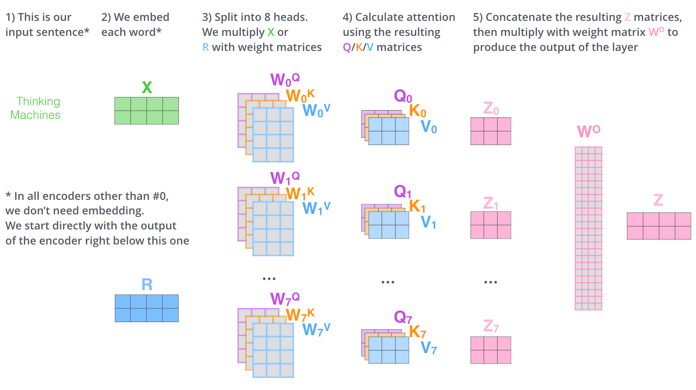
图解 Transform 中用一张图片表示了上述的计算过程:
5. 前馈层
5.1 基本的前馈层
在自注意力层之后,编码器有一个前馈神经网络 (FFN)。这是一个简单的网络,包含两个线性变换和一个 ReLU 激活函数。 图解Transform 中没有详细介绍它,所以让我简要解释一下。FFN 的目标是处理和转换注意机制产生的表示。通常的流程如下 (参见原论文的第 3.3 节):
-
第一个线性层: 通常会扩展输入的维度。例如,如果输入维度是 512,输出维度可能是 2048。这样做是为了使模型能够学习更复杂的函数。在我们的简单示例中,维度从 4 扩展到 8。
-
ReLU 激活: 这是一个非线性激活函数。它是一个简单的函数,如果输入是负数,则返回 0;如果输入是正数,则返回输入本身。这使得模型能够学习非线性函数。其数学表达如下:
ReLU(x) = \begin{cases} 0 & \text{if } x < 0 \\ x & \text{if } x \geq 0 \end{cases} -
第二个线性层: 这是第一个线性层的逆操作。它将维度降低回原始维度。在我们的示例中,维度将从 8 降低到 4。
\text{FFN}(x) = \text{ReLU}(xW_1 + b_1)W_2 + b_2
我们可以将所有这些表示如下:
注意,该层的输入是我们在上面的自注意力中计算得到的 Z:
现在让我们为权重矩阵和偏置向量定义一些随机值。我将使用代码来完成,但如果你有耐心,也可以手动完成。
W1 = np.random.randn(4, 8)
W2 = np.random.randn(8, 4)
b1 = np.random.randn(8)
b2 = np.random.randn(4)
现在让我们编写正向传递函数。
 def relu(x):
     return np.maximum(0, x)

 def feed_forward(Z, W1, b1, W2, b2):
     return relu(Z.dot(W1) + b1).dot(W2) + b2
 output_encoder = feed_forward(Z, W1, b1, W2, b2)
 output_encoder
 array([[ -3.24115016,  -9.7901049 , -29.42555675, -19.93135286],
        [ -3.40199463,  -9.87245924, -30.05715408, -20.05271018]])
5.2 全部封装起来: 随机编码器 (Random Encoder)
现在让我们编写一些代码,将多头注意力和前馈层全部放在编码器块中。
:::{.callout-note}
这段代码的优化目标是理解和学习,并非为了最佳性能!请不要过于苛刻地评判!
:::
d_embedding = 4
d_key = d_value = d_query = 3
d_feed_forward = 8
n_attention_heads = 2
def attention(x, WQ, WK, WV):
    K = x @ WK
    V = x @ WV
    Q = x @ WQ
    scores = Q @ K.T
    scores = scores / np.sqrt(d_key)
    scores = softmax(scores)
    scores = scores @ V
    return scores
def multi_head_attention(x, WQs, WKs, WVs):
    attentions = np.concatenate(
        [attention(x, WQ, WK, WV) for WQ, WK, WV in zip(WQs, WKs, WVs)], axis=1
    )
    W = np.random.randn(n_attention_heads * d_value, d_embedding)
    return attentions @ W
def feed_forward(Z, W1, b1, W2, b2):
    return relu(Z.dot(W1) + b1).dot(W2) + b2
def encoder_block(x, WQs, WKs, WVs, W1, b1, W2, b2):
    Z = multi_head_attention(x, WQs, WKs, WVs)
    Z = feed_forward(Z, W1, b1, W2, b2)
    return Z
def random_encoder_block(x):
    WQs = [
        np.random.randn(d_embedding, d_query) for _ in range(n_attention_heads)
    ]
    WKs = [
        np.random.randn(d_embedding, d_key) for _ in range(n_attention_heads)
    ]
    WVs = [
        np.random.randn(d_embedding, d_value) for _ in range(n_attention_heads)
    ]
    W1 = np.random.randn(d_embedding, d_feed_forward)
    b1 = np.random.randn(d_feed_forward)
    W2 = np.random.randn(d_feed_forward, d_embedding)
    b2 = np.random.randn(d_embedding)
    return encoder_block(x, WQs, WKs, WVs, W1, b1, W2, b2)
回想一下,我们的输入是矩阵 E,其中包含位置编码和文本嵌入。
embedding
 array([[1.  , 3.  , 3.  , 5.  ],
        [2.84, 3.99, 4.  , 6.  ]])
现在让我们将其传递给我们的 random_encoder_block 函数。
random_encoder_block(embedding)
 array([[ -71.76537515, -131.43316885,   13.2938131 ,   -4.26831998],
        [ -72.04253781, -131.84091347,   13.3385937 ,   -4.32872015]])
太棒了!这只是一个编码器块。原始论文使用了 6 个编码器。一个编码器的输出进入下一个编码器,依此类推。
 def encoder(x, n=6):
     for _ in range(n):
         x = random_encoder_block(x)
     return x


 encoder(embedding)
 /tmp/ipykernel_11906/1045810361.py:2: RuntimeWarning: overflow encountered in exp
   return np.exp(x)/np.sum(np.exp(x),axis=1, keepdims=True)
 /tmp/ipykernel_11906/1045810361.py:2: RuntimeWarning: invalid value encountered in divide
   return np.exp(x)/np.sum(np.exp(x),axis=1, keepdims=True)
 array([[nan, nan, nan, nan],
        [nan, nan, nan, nan]])
5.3 残差连接和层归一化
糟糕!我们得到了 NaN 值!看起来我们的值太大了,当传递给下一个编码器时,它们变得太大从而发散了!这被称为梯度爆炸。在没有任何归一化的情况下,早期层输入的微小变化会在后续层中被放大。这是深度神经网络中常见的问题。有两种常见的技术可以缓解这个问题: 残差连接和层归一化 (论文中第 3.1 节中简单提到)。
- 残差连接: 残差连接就是将层的输入与其输出相加。例如,我们将初始嵌入添加到注意力的输出中。残差连接可以缓解梯度消失问题。其直观理解是,如果梯度太小,我们可以将输入添加到输出中,梯度就会变大。数学上很简单:\text{Residual}(x) = x + \text{Layer}(x)
就是这样!我们将对注意力的输出和前馈层的输出都进行残差连接。
- 层归一化 (Layer normalization): 层归一化是一种对层输入进行归一化的技术。它在文本嵌入维度上进行归一化。其直观理解是,我们希望对单层的输入进行归一化,使其具有均值为 0 和标准差为 1。这有助于梯度的流动。乍一看,数学公式并不那么简单。\text{LayerNorm}(x) = \frac{x - \mu}{\sqrt{\sigma^2 + \epsilon}} \times \gamma + \beta
让我们解释一下每个参数的含义:
- \mu 是文本嵌入的均值
- \sigma 是文本嵌入的标准差
- \epsilon 是一个较小的数,用于避免除以零。如果标准差为 0,这个小的 epsilon 就派上了用场!
- \gamma 和 \beta 是可学习参数,用于控制缩放和平移。
与批归一化 (batch normalization) 不同 (如果你不知道它是什么也没关系),层归一化是在文本嵌入维度上进行归一化的,这意味着每个文本嵌入都不会受到 batch 中其他样本的影响。其直观理解是,我们希望对层的输入进行归一化,使其具有均值为 0 和标准差为 1。
为什么要添加可学习的参数 \gamma 和 \beta ?原因是我们不想失去层的表示能力。如果我们只对输入进行归一化,可能会丢失一些信息。通过添加可学习的参数,我们可以学习缩放和平移归一化后的值。
将这些方程组合起来,整个编码器的方程可能如下所示:
让我们使用之前的 E 和 Z 值尝试一下!
现在让我们计算层归一化,我们可以分为三个步骤:
- 计算每个文本嵌入的均值和方差。
- 通过减去其行的均值并除以其行方差的平方根 (加上一个小数以避免除以零) 进行归一化。
- 通过乘以 gamma 并加上 beta 进行缩放和平移。
5.3.1 均值和方差
对于第一个文本嵌入 (“Hello”):
我们可以对第二个文本嵌入 (“World”) 进行相同的操作。这里我们跳过计算步骤,但你应该能理解这个过程。
让我们用 Python 进行验证。
(embedding + Z).mean(axis=-1, keepdims=True)
 array([[-4.58837567],
        [-3.59559107]])
(embedding + Z).std(axis=-1, keepdims=True)
 array([[ 9.92061529],
        [10.50653019]])
太棒了!现在让我们进行归一化。
5.3.2 归一化
在归一化时,我们需要将文本嵌入中的每个值减去均值并除以标准差。Epsilon 是一个非常小的值,例如 0.00001。我们假设 \gamma=1 和 \beta=0 ,这样可以简化计算。
对于第二个嵌入,我们将跳过手动计算的步骤,直接用代码进行验证!让我们重新定义修改后的 encoder_block 函数。
 def layer_norm(x, epsilon=1e-6):
     mean = x.mean(axis=-1, keepdims=True)
     std = x.std(axis=-1, keepdims=True)
     return (x - mean) / (std + epsilon)

 def encoder_block(x, WQs, WKs, WVs, W1, b1, W2, b2):
     Z = multi_head_attention(x, WQs, WKs, WVs)
     Z = layer_norm(Z + x)

     output = feed_forward(Z, W1, b1, W2, b2)
     return layer_norm(output + Z)
layer_norm(Z + embedding)
 array([[ 1.71887693, -0.56365339, -0.40370747, -0.75151608],
        [ 1.71909039, -0.56050453, -0.40695381, -0.75163205]])
它输出了正确的结果!现在让我们再次将文本嵌入依次传递给六个编码器。
 def encoder(x, n=6):
     for _ in range(n):
         x = random_encoder_block(x)
     return x


 encoder(embedding)
 array([[-0.335849  , -1.44504571,  1.21698183,  0.56391289],
        [-0.33583947, -1.44504861,  1.21698606,  0.56390202]])
太棒了!这些值是有意义的,我们没有得到 NaN 值!编码器的思想是它们输出一个连续的表示 Z,捕捉输入序列的含义。然后将该表示传递给解码器,解码器将逐个生成一个个符号的输出序列。
在深入研究解码器之前,这里有一张来自 Jay 博客的结构清晰的图片:
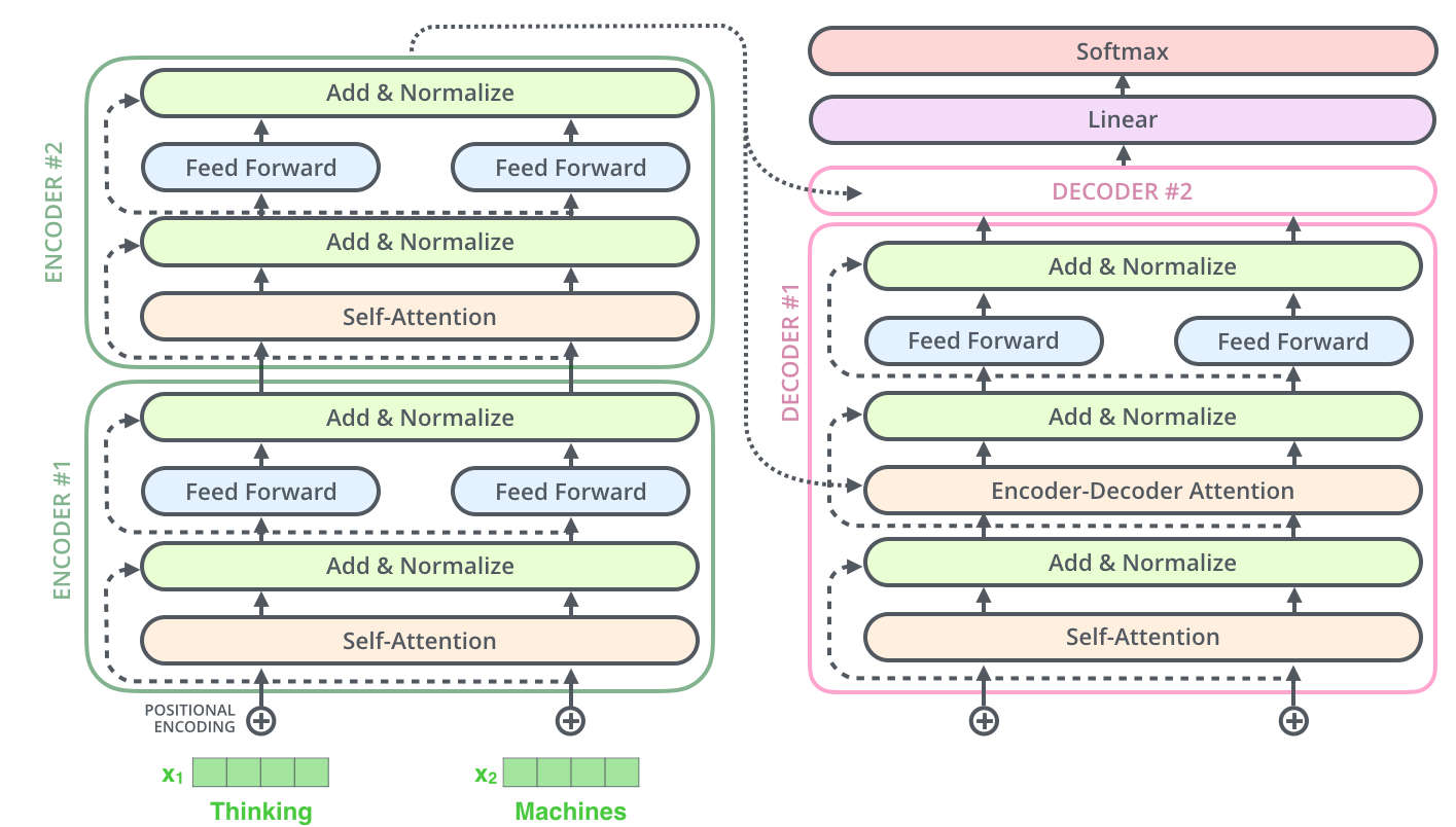
你应该能够理解左侧的每个组件!相当令人印象深刻,对吧?现在让去看看解码器。
解码器
大部分我们在编码器中学到的内容也会在解码器中使用!解码器有两个自注意力层,一个用于编码器,一个用于解码器。解码器还有一个前馈层。让我们逐个介绍一下这些内容。
解码器块接收两个输入: 编码器的输出和已经生成的解码器的输出序列。在推理过程中,将从特殊的起始序列标记 (SOS) 开始依次生成输出序列。在训练过程中,解码器需要预测目标输出序列的后一个字符并于真实的作比较。接下来我们将用一个例子来讲解这个过程!
将文本嵌入和 SOS 标记输入编码器,解码器将生成序列的下一个 token。解码器是自回归的,这意味着解码器将使用先前生成的 token 再次生成第二个 token。 (下面的例子中输出的是西班牙语)
- 迭代 1: 输入为 SOS,输出为“hola”
- 迭代 2: 输入为 SOS + “hola”,输出为“mundo”
- 迭代 3: 输入为 SOS + “hola” + “mundo”,输出为 EOS
在这里,SOS 是起始序列标记,EOS 是结束序列标记。当解码器生成 EOS 标记时,它将停止生成。它每次生成一个 token。请注意,每次的迭代过程都使用编码器生成的文本嵌入。
说明
这种自回归设计使得解码器变得很慢。 编码器能够在一次前向传递中生成其文本嵌入,而解码器需要进行多次前向传递逐个 token 生成。这是为什么仅使用编码器的架构 (如 BERT 或语义相似性模型) 比仅使用解码器的架构 (如 GPT-2 或 BART) 快得多的原因之一。
让我们深入了解每个步骤!和编码器一样,解码器由一系列解码器块组成。解码器块比编码器块稍微复杂一些。它的一般结构是:
- (带有掩码的) 自注意力层
- 残差连接和层归一化
- 编码器-解码器注意力层
- 残差连接和层归一化
- 前馈层
- 残差连接和层归一化
我们已经熟悉了 1、2、3、5 和 6 的所有数学知识。查看下面的图像右侧,相信你已经了解了这些块 (右侧部分):

1. 对文本进行嵌入
解码器的第一步是对输入 token 进行文本嵌入。第一个输入 token 是 SOS ,所以我们将对其进行文本嵌入。我们将使用与编码器相同的文本嵌入维度。假设嵌入向量如下:
2. 位置编码
现在我们为文本嵌入添加位置编码,就像我们在编码器时做的那样。由于它与“Hello”的位置相同,它有与其相同的位置编码:
- i = 0(偶数):PE(0,0) = sin(0 / 10000^(0 / 4)) = sin(0) = 0
- i = 1(奇数):PE(0,1) = cos(0 / 10000^(2*1 / 4)) = cos(0) = 1
- i = 2(偶数):PE(0,2) = sin(0 / 10000^(2*2 / 4)) = sin(0) = 0
- i = 3(奇数):PE(0,3) = cos(0 / 10000^(2*3 / 4)) = cos(0) = 1
3. 将位置编码添加到文本嵌入中
通过将这两个向量相加,将位置编码添加到文本嵌入中:
4. 自注意力
解码器块中的第一步是自注意力机制。幸运的是,我们已经之前已经写过自注意力的代码,可以直接使用!
d_embedding = 4
n_attention_heads = 2
E = np.array([[1, 1, 0, 1]])
WQs = [np.random.randn(d_embedding, d_query) for _ in range(n_attention_heads)]
WKs = [np.random.randn(d_embedding, d_key) for _ in range(n_attention_heads)]
WVs = [np.random.randn(d_embedding, d_value) for _ in range(n_attention_heads)]
Z_self_attention = multi_head_attention(E, WQs, WKs, WVs)
Z_self_attention
array([[ 2.19334924, 10.61851198, -4.50089666, -2.76366551]])
说明
对于推理来说,事情相当简单。对于训练来说,情况有点复杂。在训练过程中,我们使用无标签数据: 只是一堆文本数据,通常是从网络上抓取的。虽然编码器的目标是捕捉输入的所有信息,但解码器的目标是预测最可能的下一个 token。这意味着解码器只能使用到目前为止已经生成的 token (它不能作弊地查看下一个 token)。
因此,我们使用了带有掩码的自注意力: 我们将尚未生成的 token 屏蔽掉。这是在原始论文中的做法 (第 3.2.3.1 节)。我们暂时跳过这一步,但是要记住,在训练过程中,解码器会变得更加复杂。
5. 残差连接和层归一化
这里没有什么比较复杂的,我们只是将输入与自注意力的输出相加,并进行层归一化。我们将使用与之前相同的代码。
Z_self_attention = layer_norm(Z_self_attention + E)
Z_self_attention
array([[ 0.17236212, 1.54684892, -1.0828824 , -0.63632864]])
6. 编码器-解码器注意力
这部分的内容与之前的有所不同! 如果你想知道编码器生成的文本嵌入在哪里发挥作用,那么现在就是它们展现自己的时刻!
假设编码器的输出是以下矩阵:
在编码器的自注意力机制中,我们使用输入的文本嵌入计算 Q 矩阵 (queries)、K 矩阵 (keys) 和 V 矩阵 (values)。
在编码器-解码器注意力中,我们使用前一个解码器层计算 Q 矩阵,使用编码器输出计算 K 矩阵和 V 矩阵!所有的数学计算都与之前相同;唯一的区别是计算 Q 矩阵时使用哪个文本嵌入。让我们看一些代码:
def encoder_decoder_attention(encoder_output, attention_input, WQ, WK, WV):
    # The next three lines are the key difference!
    K = encoder_output @ WK    # Note that now we pass the previous encoder output!
    V = encoder_output @ WV    # Note that now we pass the previous encoder output!
    Q = attention_input @ WQ   # Same as self-attention
    # This stays the same
    scores = Q @ K.T
    scores = scores / np.sqrt(d_key)
    scores = softmax(scores)
    scores = scores @ V
    return scores
def multi_head_encoder_decoder_attention(
    encoder_output, attention_input, WQs, WKs, WVs
):
    # Note that now we pass the previous encoder output!
    attentions = np.concatenate(
        [
            encoder_decoder_attention(
                encoder_output, attention_input, WQ, WK, WV
            )
            for WQ, WK, WV in zip(WQs, WKs, WVs)
        ],
        axis=1,
    )
    W = np.random.randn(n_attention_heads * d_value, d_embedding)
    return attentions @ W
WQs = [np.random.randn(d_embedding, d_query) for _ in range(n_attention_heads)]
WKs = [np.random.randn(d_embedding, d_key) for _ in range(n_attention_heads)]
WVs = [np.random.randn(d_embedding, d_value) for _ in range(n_attention_heads)]
encoder_output = np.array([[-1.5, 1.0, -0.8, 1.5], [1.0, -1.0, -0.5, 1.0]])
Z_encoder_decoder = multi_head_encoder_decoder_attention(
    encoder_output, Z_self_attention, WQs, WKs, WVs
)
Z_encoder_decoder
array([[ 1.57651431, 4.92489307, -0.08644448, -0.46776051]])
这个方法有效!你可能会问: “为什么要这样做呢?”原因是我们希望解码器可以学习关注到于输入文本中与当前输出的 token 相关的部分 (例如,“hello world”)。编码器-解码器的注意力机制使得解码器的每个位置都能够获取输入序列中的所有位置的信息。这对于翻译等任务非常有帮助,因为解码器需要专注于输入序列。通过学习生成正确的输出 token,解码器将学会关注输入序列的相关部分。这就是交叉自注意力机制 (cross-attention mechanism),一个非常强大的机制!
7. 残差连接和层归一化
与之前相同!
 Z_encoder_decoder = layer_norm(Z_encoder_decoder + Z)
 Z_encoder_decoder
array([[-0.44406723, 1.6552893 , -0.19984632, -1.01137575]])
8. 前馈层
同样与之前的相同!我还会在此之后进行残差连接和层归一化。
 W1 = np.random.randn(4, 8)
 W2 = np.random.randn(8, 4)
 b1 = np.random.randn(8)
 b2 = np.random.randn(4)

 output = feed_forward(Z_encoder_decoder, W1, b1, W2, b2) + Z_encoder_decoder
 output
array([[-0.97650182, 0.81470137, -2.79122044, -3.39192873]])
9. 全部封装起来: 随机解码器 (Random Decoder)
让我们编写整个解码器模块的代码。与编码器相比主要的变化是我们现在有了一个额外的注意力机制。
d_embedding = 4
d_key = d_value = d_query = 3
d_feed_forward = 8
n_attention_heads = 2
encoder_output = np.array([[-1.5, 1.0, -0.8, 1.5], [1.0, -1.0, -0.5, 1.0]])
def decoder_block(
    x,
    encoder_output,
    WQs_self_attention, WKs_self_attention, WVs_self_attention,
    WQs_ed_attention, WKs_ed_attention, WVs_ed_attention,
    W1, b1, W2, b2,
):
    # Same as before
    Z = multi_head_attention(
        x, WQs_self_attention, WKs_self_attention, WVs_self_attention
    )
    Z = layer_norm(Z + x)
    # The next three lines are the key difference!
    Z_encoder_decoder = multi_head_encoder_decoder_attention(
        encoder_output, Z, WQs_ed_attention, WKs_ed_attention, WVs_ed_attention
    )
    Z_encoder_decoder = layer_norm(Z_encoder_decoder + Z)
    # Same as before
    output = feed_forward(Z_encoder_decoder, W1, b1, W2, b2)
    return layer_norm(output + Z_encoder_decoder)
def random_decoder_block(x, encoder_output):
    # Just a bunch of random initializations
    WQs_self_attention = [
        np.random.randn(d_embedding, d_query) for _ in range(n_attention_heads)
    ]
    WKs_self_attention = [
        np.random.randn(d_embedding, d_key) for _ in range(n_attention_heads)
    ]
    WVs_self_attention = [
        np.random.randn(d_embedding, d_value) for _ in range(n_attention_heads)
    ]
    WQs_ed_attention = [
        np.random.randn(d_embedding, d_query) for _ in range(n_attention_heads)
    ]
    WKs_ed_attention = [
        np.random.randn(d_embedding, d_key) for _ in range(n_attention_heads)
    ]
    WVs_ed_attention = [
        np.random.randn(d_embedding, d_value) for _ in range(n_attention_heads)
    ]
    W1 = np.random.randn(d_embedding, d_feed_forward)
    b1 = np.random.randn(d_feed_forward)
    W2 = np.random.randn(d_feed_forward, d_embedding)
    b2 = np.random.randn(d_embedding)
    return decoder_block(
        x, encoder_output,
        WQs_self_attention, WKs_self_attention, WVs_self_attention,
        WQs_ed_attention, WKs_ed_attention, WVs_ed_attention,
        W1, b1, W2, b2,
    )
def decoder(x, decoder_embedding, n=6):
    for _ in range(n):
        x = random_decoder_block(x, decoder_embedding)
    return x
decoder(E, encoder_output)
array([[ 0.71866458, -1.72279956, 0.57735876, 0.42677623]])
生成输出序列
我们已经有了所有的基本模块!现在让我们生成输出序列。
- 我们有编码器,它接收输入序列并生成其丰富的表示。它由一系列编码器块组成。
- 我们有解码器,它接收编码器的输出和之前生成的 token,并生成输出序列。它由一系列解码器块组成。
我们如何从解码器的输出得到一个单词呢?我们需要在解码器的顶部添加一个最终的线性层和一个 softmax 层。整个算法看起来像这样:
- 编码器接收输入序列并生成其表示。
- 解码器以 SOS 标记和编码器的输出作为起点,生成输出序列的下一个 token。
- 然后,我们使用一个线性层来生成 logits。
- 然后,我们应用一个 softmax 层来生成概率。
- 解码器使用编码器的输出和先前生成的 token 来生成输出序列的下一个 token。
- 我们重复步骤 2-5,直到生成 EOS 标记。
这在论文的第 3.4 节中提到。
1. 线性层
线性层是一个简单的线性变换。它接收解码器的输出,并将其转换为大小为 vocab_size 的向量。这个大小对应的是词汇表的大小。例如,如果我们有一个包含 10000 个单词的词汇表,线性层将解码器的输出转换为大小为 10000 的向量。这个向量将包含每个单词成为序列中下一个单词的概率。为简单起见,让我们使用一个包含 10 个单词的词汇表,并假设第一个解码器的输出是一个非常简单的向量: [1, 0, 1, 0]。我们将使用一个随机生成的权重矩阵和偏置向量,它们的大小是 vocab\_size * decoder\_output\_size 。
 def linear(x, W, b):
     return np.dot(x, W) + b

 x = linear([[1, 0, 1, 0]], np.random.randn(4, 10), np.random.randn(10))
 x
 array([[-0.39929948,  0.96345013,  2.77090264,  0.25651866, -0.84738762,
         -1.67834992, -0.29583529, -3.55515281,  2.97453801, -1.10682376]])
2. Softmax
线性层的输出被称为 logits,但它们不容易解释。我们需要使用 softmax 函数来获得概率。
softmax(x)
array([[0.01602618, 0.06261303, 0.38162024, 0.03087794, 0.0102383 ,
        0.00446011, 0.01777314, 0.00068275, 0.46780959, 0.00789871]])
我们得到了概率!让我们假设词汇表如下:
上述输出告诉我们概率为:
- hello:0.01602618
- mundo:0.06261303
- world:0.38162024
- how:0.03087794
- ?0.0102383
- EOS:0.00446011
- SOS:0.01777314
- a:0.00068275
- hola:0.46780959
- c:0.00789871
从中可以看出,最可能的下一个 token 是“hola”。每次都选择最可能的 token 称为贪婪解码。这并不总是最好的方法,因为它可能导致次优结果,但我们暂时不深入研究生成技术。如果你想了解更多信息,请查看这篇非常 amazing 的 博客文章 。
3. 随机编码器-解码器的 Transformer
让我们编写完整的代码!我们定义一个将单词映射到它们初始文本嵌入的字典。请注意,这些初始值训练过程中也是通过学习获得的,但现在我们将使用随机值。
vocabulary = [
    "hello",
    "mundo",
    "world",
    "how",
    "?",
    "EOS",
    "SOS",
    "a",
    "hola",
    "c",
]
embedding_reps = np.random.randn(10, 1, 4)
vocabulary_embeddings = {
    word: embedding_reps[i] for i, word in enumerate(vocabulary)
}
vocabulary_embeddings
{'hello': array([[-1.19489531, -1.08007463,  1.41277762,  0.72054139]]),
 'mundo': array([[-0.70265064, -0.58361306, -1.7710761 ,  0.87478862]]),
 'world': array([[ 0.52480342,  2.03519246, -0.45100608, -1.92472193]]),
 'how': array([[-1.14693176, -1.55761929,  1.09607545, -0.21673596]]),
 '?': array([[-0.23689522, -1.12496841, -0.03733462, -0.23477603]]),
 'EOS': array([[ 0.5180958 , -0.39844119,  0.30004136,  0.03881324]]),
 'SOS': array([[ 2.00439161,  2.19477149, -0.84901634, -0.89269937]]),
 'a': array([[ 1.63558337, -1.2556952 ,  1.65365362,  0.87639945]]),
 'hola': array([[-0.5805717 , -0.93861149,  1.06847734, -0.34408367]]),
 'c': array([[-2.79741142,  0.70521986, -0.44929098, -1.66167776]])}
现在让我们编写 generate 方法来自回归地生成 token。
def generate(input_sequence, max_iters=10):
    # We first encode the inputs into embeddings
    # This skips the positional encoding step for simplicity
    embedded_inputs = [
        vocabulary_embeddings[token][0] for token in input_sequence
    ]
    print("Embedding representation (encoder input)", embedded_inputs)
    # We then generate an embedding representation
    encoder_output = encoder(embedded_inputs)
    print("Embedding generated by encoder (encoder output)", encoder_output)
    # We initialize the decoder output with the embedding of the start token
    sequence = vocabulary_embeddings["SOS"]
    output = "SOS"
    # Random matrices for the linear layer
    W_linear = np.random.randn(d_embedding, len(vocabulary))
    b_linear = np.random.randn(len(vocabulary))
    # We limit number of decoding steps to avoid too long sequences without EOS
    for i in range(max_iters):
        # Decoder step
        decoder_output = decoder(sequence, encoder_output)
        logits = linear(decoder_output, W_linear, b_linear)
        probs = softmax(logits)
        # We get the most likely next token
        next_token = vocabulary[np.argmax(probs)]
        sequence = vocabulary_embeddings[next_token]
        output += " " + next_token
        print(
            "Iteration", i,
            "next token", next_token,
            "with probability of", np.max(probs),
        )
        # If the next token is the end token, we return the sequence
        if next_token == "EOS":
            return output
    return output
现在让我们运行它!
generate(["hello", "world"])
 Embedding representation (encoder input) [array([-1.19489531, -1.08007463,  1.41277762,  0.72054139]), array([ 0.52480342,  2.03519246, -0.45100608, -1.92472193])]
 Embedding generated by encoder (encoder output) [[-0.15606365  0.90444064  0.82531037 -1.57368737]
  [-0.15606217  0.90443936  0.82531082 -1.57368802]]
 Iteration 0 next token how with probability of 0.6265258176587956
 Iteration 1 next token a with probability of 0.42708031743571
 Iteration 2 next token c with probability of 0.44288777368698484
'SOS how a c'
好的,我们得到了“how”、“a”和“c”这些 token。这不是一个好的翻译,但可以理解!因为我们只使用了随机权重!
我建议你再次详细研究原始论文中的整个编码器-解码器架构:
结论
希望这篇文章有趣且有益!我们涵盖了很多内容。等等,这就结束了吗?答案是,大部分是的!新的 Transformer 架构添加了许多技巧,但 Transformer 的核心就是我们刚刚讲解的内容。根据你想解决的任务,你也可以只使用编码器或解码器。例如,对于以理解为重的任务 (如分类),你可以使用堆叠的编码器和一个线性层。对于以生成为重的任务 (如翻译),你可以使用编码器和堆叠的解码器。最后,对于自由生成,如 ChatGPT 或 Mistral,你可以只使用堆叠的解码器。
当然,我们也做了很多简化。让我们简要地看一下原始 Transformer 论文中的一些数字:
- 文本嵌入维度: 512 (在我们的例子中为 4)
- 编码器数量: 6 (在我们的例子中为 6)
- 解码器数量: 6 (在我们的例子中为 6)
- 前馈维度: 2048 (在我们的例子中为 8)
- 注意力头数: 8 (在我们的例子中为 2)
- 注意力维度: 64 (在我们的例子中为 3)
我们刚刚涵盖了很多主题,通过扩展模型的大小并进行智能训练,我们可以实现令人印象深刻的结果。由于本文的目标是理解现有模型的数学原理,所以我们没有涉及模型训练部分,但我希望能够为学习模型训练部分提供坚实的基础。希望你喜欢这篇博文!
练习
以下是一些练习,以检验你对 Transformer 的理解。
- 位置编码的目的是什么?
- 自注意力和编码器-解码器注意力有什么区别?
- 如果我们的注意力维度太小会发生什么?如果太大呢?
- 简要描述一下前馈层的结构。
- 为什么解码器比编码器慢?
- 残差连接和层归一化的目的是什么?
- 我们如何从解码器的输出得到概率?
- 为什么每次都选择最可能的下一个 token 会带来问题?
资源
原文: hackerllama - The Random Transformer
作者: Omar Sanseviero
译者: yaoqih