在《使用 ![]() Transformers 进行概率时间序列预测》的第一部分里,我们为大家介绍了传统时间序列预测和基于 Transformers 的方法,也一步步准备好了训练所需的数据集并定义了环境、模型、转换和
Transformers 进行概率时间序列预测》的第一部分里,我们为大家介绍了传统时间序列预测和基于 Transformers 的方法,也一步步准备好了训练所需的数据集并定义了环境、模型、转换和 InstanceSplitter。本篇内容将包含从数据加载器,到前向传播、训练、推理和展望未来发展等精彩内容。
创建 PyTorch 数据加载器
有了数据,下一步需要创建 PyTorch DataLoaders。它允许我们批量处理成对的 (输入, 输出) 数据,即 (past_values , future_values)。
from gluonts.itertools import Cyclic, IterableSlice, PseudoShuffled
from gluonts.torch.util import IterableDataset
from torch.utils.data import DataLoader

from typing import Iterable

def create_train_dataloader(
    config: PretrainedConfig,
    freq,
    data,
    batch_size: int,
    num_batches_per_epoch: int,
    shuffle_buffer_length: Optional[int] = None,
    **kwargs,
) -> Iterable:
    PREDICTION_INPUT_NAMES = [
        "static_categorical_features",
        "static_real_features",
        "past_time_features",
        "past_values",
        "past_observed_mask",
        "future_time_features",
        ]

    TRAINING_INPUT_NAMES = PREDICTION_INPUT_NAMES + [
        "future_values",
        "future_observed_mask",
        ]

    transformation = create_transformation(freq, config)
    transformed_data = transformation.apply(data, is_train=True)

    # we initialize a Training instance
    instance_splitter = create_instance_splitter(
        config, "train"
    ) + SelectFields(TRAINING_INPUT_NAMES)


    # the instance splitter will sample a window of
    # context length + lags + prediction length (from the 366 possible transformed time series)
    # randomly from within the target time series and return an iterator.
    training_instances = instance_splitter.apply(
        Cyclic(transformed_data)
        if shuffle_buffer_length is None
        else PseudoShuffled(
            Cyclic(transformed_data),
            shuffle_buffer_length=shuffle_buffer_length,
        )
    )

    # from the training instances iterator we now return a Dataloader which will
    # continue to sample random windows for as long as it is called
    # to return batch_size of the appropriate tensors ready for training!
    return IterableSlice(
        iter(
            DataLoader(
                IterableDataset(training_instances),
                batch_size=batch_size,
                **kwargs,
            )
        ),
        num_batches_per_epoch,
    )
def create_test_dataloader(
    config: PretrainedConfig,
    freq,
    data,
    batch_size: int,
    **kwargs,
):
    PREDICTION_INPUT_NAMES = [
        "static_categorical_features",
        "static_real_features",
        "past_time_features",
        "past_values",
        "past_observed_mask",
        "future_time_features",
        ]

    transformation = create_transformation(freq, config)
    transformed_data = transformation.apply(data, is_train=False)

    # we create a Test Instance splitter which will sample the very last
    # context window seen during training only for the encoder.
    instance_splitter = create_instance_splitter(
        config, "test"
    ) + SelectFields(PREDICTION_INPUT_NAMES)

    # we apply the transformations in test mode
    testing_instances = instance_splitter.apply(transformed_data, is_train=False)

    # This returns a Dataloader which will go over the dataset once.
    return DataLoader(IterableDataset(testing_instances), batch_size=batch_size, **kwargs)
train_dataloader = create_train_dataloader(
    config=config,
    freq=freq,
    data=train_dataset,
    batch_size=256,
    num_batches_per_epoch=100,
)

test_dataloader = create_test_dataloader(
    config=config,
    freq=freq,
    data=test_dataset,
    batch_size=64,
)
让我们检查第一批:
batch = next(iter(train_dataloader))
for k,v in batch.items():
  print(k,v.shape, v.type())

>>> static_categorical_features torch.Size([256, 1]) torch.LongTensor
    static_real_features torch.Size([256, 1]) torch.FloatTensor
    past_time_features torch.Size([256, 181, 2]) torch.FloatTensor
    past_values torch.Size([256, 181]) torch.FloatTensor
    past_observed_mask torch.Size([256, 181]) torch.FloatTensor
    future_time_features torch.Size([256, 24, 2]) torch.FloatTensor
    future_values torch.Size([256, 24]) torch.FloatTensor
    future_observed_mask torch.Size([256, 24]) torch.FloatTensor
可以看出,我们没有将 input_ids 和 attention_mask 提供给编码器 (训练 NLP 模型时也是这种情况),而是提供 past_values,以及 past_observed_mask、past_time_features、static_categorical_features 和 static_real_features 几项数据。
解码器的输入包括 future_values、future_observed_mask 和 future_time_features。 future_values 可以看作等同于 NLP 训练中的 decoder_input_ids。
我们可以参考 Time Series Transformer 文档 以获得对它们中每一个的详细解释。
前向传播
让我们对刚刚创建的批次执行一次前向传播:
# perform forward pass
outputs = model(
    past_values=batch["past_values"],
    past_time_features=batch["past_time_features"],
    past_observed_mask=batch["past_observed_mask"],
    static_categorical_features=batch["static_categorical_features"],
    static_real_features=batch["static_real_features"],
    future_values=batch["future_values"],
    future_time_features=batch["future_time_features"],
    future_observed_mask=batch["future_observed_mask"],
    output_hidden_states=True
)
print("Loss:", outputs.loss.item())

>>> Loss: 9.141253471374512
目前,该模型返回了损失值。这是由于解码器会自动将 future_values 向右移动一个位置以获得标签。这允许计算预测结果和标签值之间的误差。
另请注意,解码器使用 Causal Mask 来避免预测未来,因为它需要预测的值在 future_values 张量中。
训练模型
是时候训练模型了!我们将使用标准的 PyTorch 训练循环。
这里我们用到了 ![]() Accelerate 库,它会自动将模型、优化器和数据加载器放置在适当的
Accelerate 库,它会自动将模型、优化器和数据加载器放置在适当的 device 上。
from accelerate import Accelerator
from torch.optim import Adam

accelerator = Accelerator()
device = accelerator.device

model.to(device)
optimizer = Adam(model.parameters(), lr=1e-3)

model, optimizer, train_dataloader = accelerator.prepare(
    model, optimizer, train_dataloader,
)

for epoch in range(40):
    model.train()
    for batch in train_dataloader:
        optimizer.zero_grad()
        outputs = model(
            static_categorical_features=batch["static_categorical_features"].to(device),
            static_real_features=batch["static_real_features"].to(device),
            past_time_features=batch["past_time_features"].to(device),
            past_values=batch["past_values"].to(device),
            future_time_features=batch["future_time_features"].to(device),
            future_values=batch["future_values"].to(device),
            past_observed_mask=batch["past_observed_mask"].to(device),
            future_observed_mask=batch["future_observed_mask"].to(device),
        )
        loss = outputs.loss

        # Backpropagation
        accelerator.backward(loss)
        optimizer.step()

        print(loss.item())
推理
在推理时,建议使用 generate() 方法进行自回归生成,类似于 NLP 模型。
预测的过程会从测试实例采样器中获得数据。采样器会将数据集的每个时间序列的最后 context_length 那么长时间的数据采样出来,然后输入模型。请注意,这里需要把提前已知的 future_time_features 传递给解码器。
该模型将从预测分布中自回归采样一定数量的值,并将它们传回解码器最终得到预测输出:
model.eval()

forecasts = []

for batch in test_dataloader:
    outputs = model.generate(
        static_categorical_features=batch["static_categorical_features"].to(device),
        static_real_features=batch["static_real_features"].to(device),
        past_time_features=batch["past_time_features"].to(device),
        past_values=batch["past_values"].to(device),
        future_time_features=batch["future_time_features"].to(device),
        past_observed_mask=batch["past_observed_mask"].to(device),
    )
    forecasts.append(outputs.sequences.cpu().numpy())
该模型输出一个表示结构的张量 (batch_size, number of samples, prediction length)。
下面的输出说明: 对于大小为 64 的批次中的每个示例,我们将获得接下来 24 个月内的 100 个可能的值:
forecasts[0].shape

>>> (64, 100, 24)
我们将垂直堆叠它们,以获得测试数据集中所有时间序列的预测:
forecasts = np.vstack(forecasts)
print(forecasts.shape)

>>> (366, 100, 24)
我们可以根据测试集中存在的样本值,根据真实情况评估生成的预测。这里我们使用数据集中的每个时间序列的 MASE 和 sMAPE 指标 (metrics) 来评估:
from evaluate import load
from gluonts.time_feature import get_seasonality

mase_metric = load("evaluate-metric/mase")
smape_metric = load("evaluate-metric/smape")

forecast_median = np.median(forecasts, 1)

mase_metrics = []
smape_metrics = []
for item_id, ts in enumerate(test_dataset):
    training_data = ts["target"][:-prediction_length]
    ground_truth = ts["target"][-prediction_length:]
    mase = mase_metric.compute(
        predictions=forecast_median[item_id],
        references=np.array(ground_truth),
        training=np.array(training_data),
        periodicity=get_seasonality(freq))
    mase_metrics.append(mase["mase"])

    smape = smape_metric.compute(
        predictions=forecast_median[item_id],
        references=np.array(ground_truth),
    )
    smape_metrics.append(smape["smape"])
print(f"MASE: {np.mean(mase_metrics)}")

>>> MASE: 1.361636922541396

print(f"sMAPE: {np.mean(smape_metrics)}")

>>> sMAPE: 0.17457818831512306
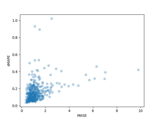
我们还可以单独绘制数据集中每个时间序列的结果指标,并观察到其中少数时间序列对最终测试指标的影响很大:
plt.scatter(mase_metrics, smape_metrics, alpha=0.3)
plt.xlabel("MASE")
plt.ylabel("sMAPE")
plt.show()
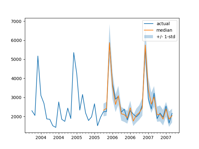
为了根据基本事实测试数据绘制任何时间序列的预测,我们定义了以下辅助绘图函数:
import matplotlib.dates as mdates

def plot(ts_index):
    fig, ax = plt.subplots()

    index = pd.period_range(
        start=test_dataset[ts_index][FieldName.START],
        periods=len(test_dataset[ts_index][FieldName.TARGET]),
        freq=freq,
    ).to_timestamp()

    # Major ticks every half year, minor ticks every month,
    ax.xaxis.set_major_locator(mdates.MonthLocator(bymonth=(1, 7)))
    ax.xaxis.set_minor_locator(mdates.MonthLocator())

    ax.plot(
        index[-2*prediction_length:],
        test_dataset[ts_index]["target"][-2*prediction_length:],
        label="actual",
    )

    plt.plot(
        index[-prediction_length:],
        np.median(forecasts[ts_index], axis=0),
        label="median",
    )

    plt.fill_between(
        index[-prediction_length:],
        forecasts[ts_index].mean(0) - forecasts[ts_index].std(axis=0),
        forecasts[ts_index].mean(0) + forecasts[ts_index].std(axis=0),
        alpha=0.3,
        interpolate=True,
        label="+/- 1-std",
    )
    plt.legend()
    plt.show()
例如:
plot(334)
我们如何与其他模型进行比较? Monash Time Series Repository 有一个测试集 MASE 指标的比较表。我们可以将自己的结果添加到其中作比较:
| Dataset | SES | Theta | TBATS | ETS | (DHR-)ARIMA | PR | CatBoost | FFNN | DeepAR | N-BEATS | WaveNet | Transformer (Our) |
|---|---|---|---|---|---|---|---|---|---|---|---|---|
| Tourism Monthly | 3.306 | 1.649 | 1.751 | 1.526 | 1.589 | 1.678 | 1.699 | 1.582 | 1.409 | 1.574 | 1.482 | 1.361 |
请注意,我们的模型击败了所有已知的其他模型 (另请参见相应 论文 中的表 2) ,并且我们没有做任何超参数优化。我们仅仅花了 40 个完整训练调参周期来训练 Transformer。
当然,我们应该谦虚。从历史发展的角度来看,现在认为神经网络解决时间序列预测问题是正途,就好比当年的论文得出了 “你需要的就是 XGBoost” 的结论。我们只是很好奇,想看看神经网络能带我们走多远,以及 Transformer 是否会在这个领域发挥作用。这个特定的数据集似乎表明它绝对值得探索。
下一步
我们鼓励读者尝试我们的 Jupyter Notebook 和来自 Hugging Face Hub 的其他时间序列数据集,并替换适当的频率和预测长度参数。对于您的数据集,需要将它们转换为 GluonTS 的惯用格式,在他们的 文档 里有非常清晰的说明。我们还准备了一个示例 Notebook,向您展示如何将数据集转换为 ![]() Hugging Face 数据集格式。
Hugging Face 数据集格式。
正如时间序列研究人员所知,人们对“将基于 Transformer 的模型应用于时间序列”问题很感兴趣。传统 vanilla Transformer 只是众多基于注意力 (Attention) 的模型之一,因此需要向库中补充更多模型。
目前没有什么能妨碍我们继续探索对多变量时间序列 (multivariate time series) 进行建模,但是为此需要使用多变量分布头 (multivariate distribution head) 来实例化模型。目前已经支持了对角独立分布 (diagonal independent distributions),后续会增加其他多元分布支持。请继续关注未来的博客文章以及其中的教程。
路线图上的另一件事是时间序列分类。这需要将带有分类头的时间序列模型添加到库中,例如用于异常检测这类任务。
当前的模型会假设日期时间和时间序列值都存在,但在现实中这可能不能完全满足。例如 WOODS 给出的神经科学数据集。因此,我们还需要对当前模型进行泛化,使某些输入在整个流水线中可选。
最后,NLP/CV 领域从大型预训练模型 中获益匪浅,但据我们所知,时间序列领域并非如此。基于 Transformer 的模型似乎是这一研究方向的必然之选,我们迫不及待地想看看研究人员和从业者会发现哪些突破!
英文原文: Probabilistic Time Series Forecasting with
Transformers
译者、排版: zhongdongy (阿东)